4 Calculate Spatial Metrics
While we’ve generated some nice visualizations, we need insights quantified as metrics at the neighborhood level. Don’t start this step until you have a good idea of what you need. Visualizing and exploring the data in depth is best practice.
For our purposes, we’re interested in developing spatial access metrics with a container method approach. At the end of this tutorial, we’ll generate the following new variables:
- Total number of Methadone Maintenance MOUD by zip code
- Total number of Walkble MOUD Service Areas by zip code
Plus, we will have a new spatial layer, that includes the actual service areas (ie. 1-mile buffers of MOUDs). We assume that access to MOUDs is critical and requires high regularity, and that walking is the most likely option during COVID. This guides the parameter specification of MOUD Service Areas (and is also backed up by some literature in this space, though much more is needed.)
4.1 Load Spatial Data
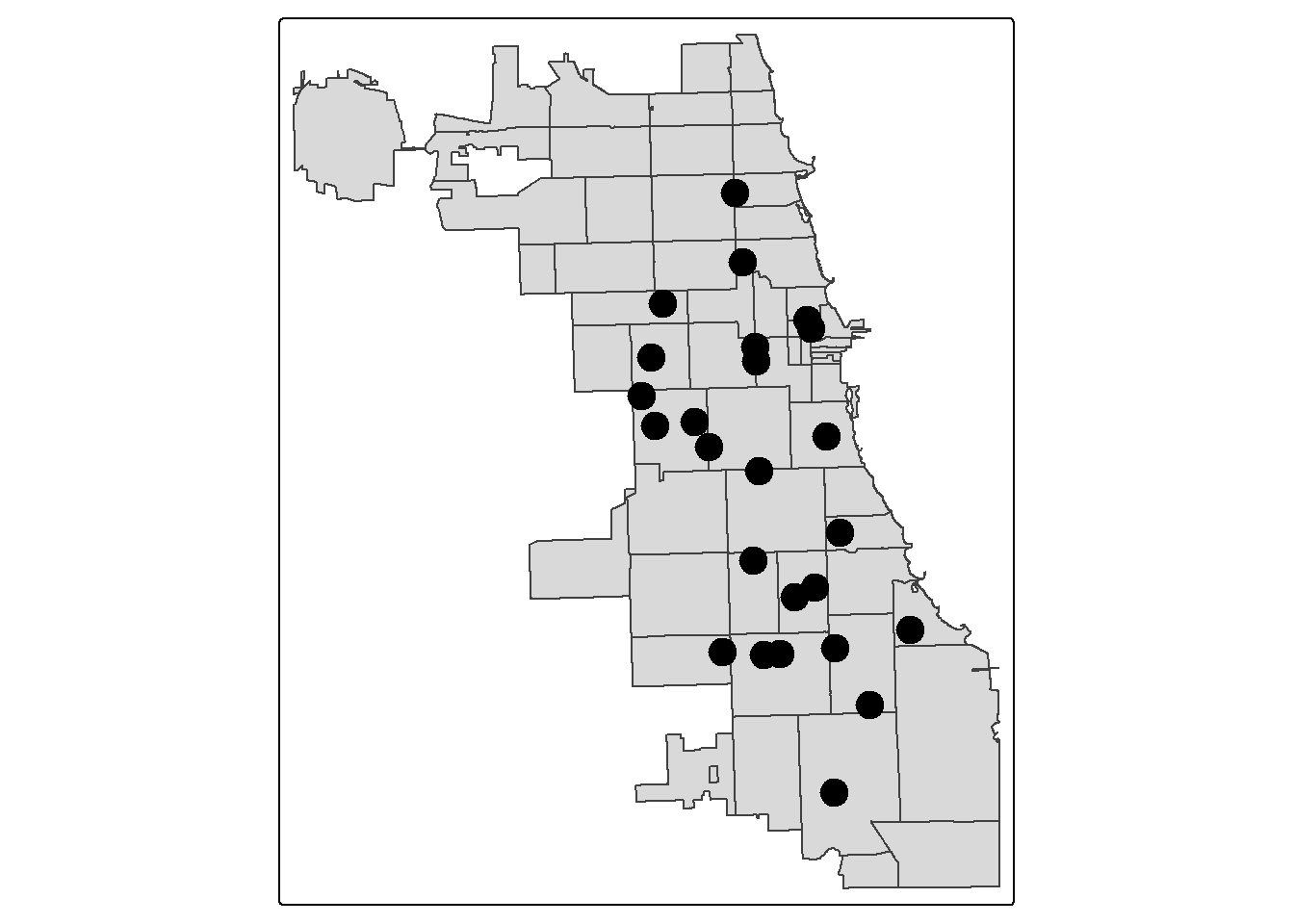
Let’s first reload our spatial data – this will be the MOUD points, plus the master zip code spatial file.
## Reading layer `methadoneMOUD' from data source `C:\Users\wimer\github\oeps\Spatial-Health-Workshop\data\methadoneMOUD.geojson'
##   using driver `GeoJSON'
## Simple feature collection with 25 features and 8 fields
## Geometry type: POINT
## Dimension:     XY
## Bounding box:  xmin: -87.7349 ymin: 41.68698 xmax: -87.57673 ymax: 41.9533
## Geodetic CRS: WGS 84## Reading layer `ChiZipMaster' from data source `C:\Users\wimer\github\oeps\Spatial-Health-Workshop\data\ChiZipMaster.geojson'
## using driver `GeoJSON'
## Simple feature collection with 60 features and 31 fields (with 1 geometry empty)
## Geometry type: MULTIPOLYGON
## Dimension: XY
## Bounding box: xmin: -87.94011 ymin: 41.64454 xmax: -87.52414 ymax: 42.02304
## Geodetic CRS: WGS 84## [1] 25 9## [1] 60 32## Simple feature collection with 6 features and 8 fields
## Geometry type: POINT
## Dimension: XY
## Bounding box: xmin: -87.72186 ymin: 41.88474 xmax: -87.63409 ymax: 41.9533
## Geodetic CRS: WGS 84
## X
## 1 3
## 2 4
## 3 5
## 4 6
## 5 7
## 6 8
## Name
## 1 Soft Landing Interventions/DBA Symetria Recovery of Lakeview
## 2 PDSSC - Chicago, Inc.
## 3 Center for Addictive Problems, Inc.
## 4 Family Guidance Centers, Inc.
## 5 A Rincon Family Services
## 6 *
## Address City State Zip
## 1 3934 N. Lincoln Ave. Chicago IL 60613
## 2 2260 N. Elston Ave. Chicago IL 60614
## 3 609 N. Wells St. Chicago IL 60654
## 4 310 W. Chicago Ave. Chicago IL 60654
## 5 3809 W. Grand Ave. Chicago IL 60651
## 6 140 N. Ashland Ave. Chicago IL 60607
## fullAdd
## 1 3934 N. Lincoln Ave. Chicago IL 60613
## 2 2260 N. Elston Ave. Chicago IL 60614
## 3 609 N. Wells St. Chicago IL 60654
## 4 310 W. Chicago Ave. Chicago IL 60654
## 5 3809 W. Grand Ave. Chicago IL 60651
## 6 140 N. Ashland Ave. Chicago IL 60607
## geo_method geometry
## 1 census POINT (-87.67818 41.9533)
## 2 census POINT (-87.67407 41.92269)
## 3 census POINT (-87.63409 41.89268)
## 4 census POINT (-87.63636 41.89657)
## 5 census POINT (-87.72186 41.90435)
## 6 osm POINT (-87.66725 41.88474)## Simple feature collection with 6 features and 31 fields
## Geometry type: MULTIPOLYGON
## Dimension: XY
## Bounding box: xmin: -87.63999 ymin: 41.85317 xmax: -87.60246 ymax: 41.88913
## Geodetic CRS: WGS 84
## zip objectid shape_area shape_len
## 1 60601 27 9166246 19804.58
## 2 60602 26 4847125 14448.17
## 3 60603 19 4560229 13672.68
## 4 60604 48 4294902 12245.81
## 5 60605 20 36301276 37973.35
## 6 60606 31 6766411 12040.44
## Case.Rate...Cumulative year totPopE
## 1 1451.4 2018 14675
## 2 1688.1 2018 1244
## 3 1107.3 2018 1174
## 4 3964.2 2018 782
## 5 1420.8 2018 27519
## 6 2289.6 2018 3101
## whiteP blackP amIndP asianP pacIsP otherP
## 1 74.17 5.57 0.45 18.00 0.00 1.81
## 2 68.17 3.78 5.31 19.45 0.00 3.30
## 3 63.46 3.24 0.00 27.60 0.00 5.71
## 4 63.43 5.63 0.00 29.67 0.00 1.28
## 5 61.20 17.18 0.18 16.10 0.03 5.31
## 6 72.75 2.35 0.00 18.09 0.00 6.80
## hispP noHSP age0_4 age5_14 age15_19
## 1 8.68 0.00 550 156 907
## 2 6.51 0.00 61 87 18
## 3 9.80 0.00 13 43 179
## 4 4.35 0.00 12 7 52
## 5 5.84 2.39 837 1279 2172
## 6 6.29 0.73 57 44 0
## age20_24 age15_44 age45_49 age50_54
## 1 909 8726 976 1009
## 2 91 987 46 53
## 3 172 684 75 47
## 4 168 450 27 47
## 5 2282 16364 1766 1520
## 6 139 1863 213 153
## age55_59 age60_64 ageOv65 ageOv18
## 1 324 859 2075 13855
## 2 0 5 5 1095
## 3 150 50 112 1118
## 4 54 92 93 744
## 5 1824 1360 2569 25259
## 6 168 172 431 3000
## age18_64 a15_24P und45P ovr65P disbP
## 1 11780 12.37 64.27 14.14 6.4
## 2 1090 8.76 91.24 0.40 0.2
## 3 1006 29.90 63.03 9.54 7.3
## 4 651 28.13 59.97 11.89 4.1
## 5 22690 16.19 67.15 9.34 5.3
## 6 2569 4.48 63.33 13.90 1.9
## geometry
## 1 MULTIPOLYGON (((-87.62271 4...
## 2 MULTIPOLYGON (((-87.60997 4...
## 3 MULTIPOLYGON (((-87.61633 4...
## 4 MULTIPOLYGON (((-87.63376 4...
## 5 MULTIPOLYGON (((-87.62064 4...
## 6 MULTIPOLYGON (((-87.63397 4...4.2 Transform Projections
First we need to switch to a projection that uses distance in feet or meters as a metric. We’ll use EPSG:3435 from the first tutorial. To find which EPSG was recommended, I searched “EPSG Illinois feet” and EPSG:3435 came up as a viable candidate. So, we use that for our new, projected CRS.
We may want to once again confirm they are plotting correctly:
4.3 Count resources by area
One way of understanding resource inequity is by thinking about how many resources exist in a neighborhood.
First, give the points the attributes of the polygons they are in. Inspect.
## Simple feature collection with 6 features and 39 fields
## Geometry type: POINT
## Dimension:     XY
## Bounding box:  xmin: 1150707 ymin: 1901294 xmax: 1174632 ymax: 1926255
## Projected CRS: NAD83 / Illinois East (ftUS)
##   X
## 1 3
## 2 4
## 3 5
## 4 6
## 5 7
## 6 8
##                                                           Name
## 1 Soft Landing Interventions/DBA Symetria Recovery of Lakeview
## 2                                        PDSSC - Chicago, Inc.
## 3                          Center for Addictive Problems, Inc.
## 4                                Family Guidance Centers, Inc.
## 5                                     A Rincon Family Services
## 6                                                            *
##                Address    City State   Zip
## 1 3934 N. Lincoln Ave. Chicago    IL 60613
## 2  2260 N. Elston Ave. Chicago    IL 60614
## 3     609 N. Wells St. Chicago    IL 60654
## 4  310 W. Chicago Ave. Chicago    IL 60654
## 5   3809 W. Grand Ave. Chicago    IL 60651
## 6  140 N. Ashland Ave. Chicago    IL 60607
##                                 fullAdd
## 1 3934 N. Lincoln Ave. Chicago IL 60613
## 2  2260 N. Elston Ave. Chicago IL 60614
## 3     609 N. Wells St. Chicago IL 60654
## 4  310 W. Chicago Ave. Chicago IL 60654
## 5   3809 W. Grand Ave. Chicago IL 60651
## 6  140 N. Ashland Ave. Chicago IL 60607
##   geo_method   zip objectid shape_area
## 1     census 60613       53   53990895
## 2     census 60614       32   94460632
## 3     census 60654       55   15869961
## 4     census 60610       54   31598157
## 5     census 60651       37   99039621
## 6        osm 60612       16  106718949
##   shape_len Case.Rate...Cumulative year
## 1  31196.32                 1572.4 2018
## 2  50587.35                 1604.3 2018
## 3  17119.70                 1876.1 2018
## 4  24208.70                 1706.9 2018
## 5  47970.14                 4027.3 2018
## 6  42663.20                 2885.4 2018
##   totPopE whiteP blackP amIndP asianP
## 1   50113  81.90   5.79   0.41   6.60
## 2   71308  84.61   4.01   0.03   7.45
## 3   19135  77.70   5.44   0.28  12.58
## 4   39019  73.82  14.96   0.28   8.17
## 5   63218  16.69  52.06   0.27   0.48
## 6   34311  27.72  60.48   0.19   4.65
##   pacIsP otherP hispP noHSP age0_4 age5_14
## 1   0.02   5.27 11.30  3.42   2555    2633
## 2   0.03   3.87  6.05  2.00   3908    5030
## 3   0.00   4.01  5.21  1.18   1164     423
## 4   0.00   2.77  6.67  3.84   1845    1279
## 5   0.00  30.49 42.49 24.52   4780    9228
## 6   0.16   6.81 12.26 15.57   2385    4253
##   age15_19 age20_24 age15_44 age45_49
## 1      777     5875    30790     2880
## 2     3288     8317    44016     3816
## 3       81     1163    12429     1021
## 4     1261     2997    22220     2072
## 5     4815     5255    27618     3719
## 6     2569     3295    17535     1682
##   age50_54 age55_59 age60_64 ageOv65
## 1     2546     2412     1868    4429
## 2     2769     3001     2589    6179
## 3     1352      865      754    1127
## 4     1635     1734     2205    6029
## 5     3906     3485     3262    7220
## 6     2028     1861     1431    3136
##   ageOv18 age18_64 a15_24P und45P ovr65P
## 1   44320    39891   13.27  71.79   8.84
## 2   61384    55205   16.27  74.26   8.67
## 3   17524    16397    6.50  73.25   5.89
## 4   35454    29425   10.91  64.95  15.45
## 5   45889    38669   15.93  65.85  11.42
## 6   26151    23015   17.09  70.45   9.14
##   disbP                geometry
## 1   7.2 POINT (1162460 1926255)
## 2   4.5 POINT (1163663 1915110)
## 3   4.4 POINT (1174632 1904257)
## 4   7.7 POINT (1174003 1905671)
## 5  14.7 POINT (1150707 1908328)
## 6  13.6 POINT (1165627 1901294)
You should have the same number of rows in pipr as you do in points. If not, there is something off. You may need to go back to troubleshoot. In an earlier version of this lab, I used a saved, written geojson file of the zip codes, and it would not render properly. Here, we load in the original shapefile at the beginning of the tutorial to avoid that error.
## [1] 25 40## [1] 25 9## [1] 60 324.3.1 Count # per Area
Next, count the number per area. The frequency should be logical according to the map you made earlier. Sometimes, I’ve found bugs where the numbers are multipled by some factor; this can be checked by looking at dimension disparities, as noted above.
##    Var1 Freq
## 1 60607    2
## 2 60608    1
## 3 60609    1
## 4 60613    1
## 5 60614    1
## 6 60615    1
How could improve on this step if you used dplyr?
Aggregation Tip: What if you have an attribute value you’d like to aggregate? For example, average units of affordable housing facility by zip?
Try aggregate(pip$attribute, by = list(pip$geoid), mean) but build on with a tidy sensibility…
Now we can rename our attributes:
##     zip MetClnc
## 1 60607       2
## 2 60608       1
## 3 60609       1
## 4 60613       1
## 5 60614       1
## 6 60615       1
And finally, merge back to your master zip file:
## Simple feature collection with 6 features and 31 fields
## Geometry type: MULTIPOLYGON
## Dimension:     XY
## Bounding box:  xmin: 1173038 ymin: 1889918 xmax: 1183259 ymax: 1902959
## Projected CRS: NAD83 / Illinois East (ftUS)
##     zip objectid shape_area shape_len
## 1 60601       27    9166246  19804.58
## 2 60602       26    4847125  14448.17
## 3 60603       19    4560229  13672.68
## 4 60604       48    4294902  12245.81
## 5 60605       20   36301276  37973.35
## 6 60606       31    6766411  12040.44
##   Case.Rate...Cumulative year totPopE
## 1                 1451.4 2018   14675
## 2                 1688.1 2018    1244
## 3                 1107.3 2018    1174
## 4                 3964.2 2018     782
## 5                 1420.8 2018   27519
## 6                 2289.6 2018    3101
##   whiteP blackP amIndP asianP pacIsP otherP
## 1  74.17   5.57   0.45  18.00   0.00   1.81
## 2  68.17   3.78   5.31  19.45   0.00   3.30
## 3  63.46   3.24   0.00  27.60   0.00   5.71
## 4  63.43   5.63   0.00  29.67   0.00   1.28
## 5  61.20  17.18   0.18  16.10   0.03   5.31
## 6  72.75   2.35   0.00  18.09   0.00   6.80
##   hispP noHSP age0_4 age5_14 age15_19
## 1  8.68  0.00    550     156      907
## 2  6.51  0.00     61      87       18
## 3  9.80  0.00     13      43      179
## 4  4.35  0.00     12       7       52
## 5  5.84  2.39    837    1279     2172
## 6  6.29  0.73     57      44        0
##   age20_24 age15_44 age45_49 age50_54
## 1      909     8726      976     1009
## 2       91      987       46       53
## 3      172      684       75       47
## 4      168      450       27       47
## 5     2282    16364     1766     1520
## 6      139     1863      213      153
##   age55_59 age60_64 ageOv65 ageOv18
## 1      324      859    2075   13855
## 2        0        5       5    1095
## 3      150       50     112    1118
## 4       54       92      93     744
## 5     1824     1360    2569   25259
## 6      168      172     431    3000
##   age18_64 a15_24P und45P ovr65P disbP
## 1    11780   12.37  64.27  14.14   6.4
## 2     1090    8.76  91.24   0.40   0.2
## 3     1006   29.90  63.03   9.54   7.3
## 4      651   28.13  59.97  11.89   4.1
## 5    22690   16.19  67.15   9.34   5.3
## 6     2569    4.48  63.33  13.90   1.9
##                         geometry
## 1 MULTIPOLYGON (((1177742 190...
## 2 MULTIPOLYGON (((1181226 190...
## 3 MULTIPOLYGON (((1179499 190...
## 4 MULTIPOLYGON (((1174763 189...
## 5 MULTIPOLYGON (((1178341 189...
## 6 MULTIPOLYGON (((1174681 190...## Simple feature collection with 6 features and 32 fields
## Geometry type: MULTIPOLYGON
## Dimension: XY
## Bounding box: xmin: 1173038 ymin: 1889918 xmax: 1183259 ymax: 1902959
## Projected CRS: NAD83 / Illinois East (ftUS)
## zip objectid shape_area shape_len
## 1 60601 27 9166246 19804.58
## 2 60602 26 4847125 14448.17
## 3 60603 19 4560229 13672.68
## 4 60604 48 4294902 12245.81
## 5 60605 20 36301276 37973.35
## 6 60606 31 6766411 12040.44
## Case.Rate...Cumulative year totPopE
## 1 1451.4 2018 14675
## 2 1688.1 2018 1244
## 3 1107.3 2018 1174
## 4 3964.2 2018 782
## 5 1420.8 2018 27519
## 6 2289.6 2018 3101
## whiteP blackP amIndP asianP pacIsP otherP
## 1 74.17 5.57 0.45 18.00 0.00 1.81
## 2 68.17 3.78 5.31 19.45 0.00 3.30
## 3 63.46 3.24 0.00 27.60 0.00 5.71
## 4 63.43 5.63 0.00 29.67 0.00 1.28
## 5 61.20 17.18 0.18 16.10 0.03 5.31
## 6 72.75 2.35 0.00 18.09 0.00 6.80
## hispP noHSP age0_4 age5_14 age15_19
## 1 8.68 0.00 550 156 907
## 2 6.51 0.00 61 87 18
## 3 9.80 0.00 13 43 179
## 4 4.35 0.00 12 7 52
## 5 5.84 2.39 837 1279 2172
## 6 6.29 0.73 57 44 0
## age20_24 age15_44 age45_49 age50_54
## 1 909 8726 976 1009
## 2 91 987 46 53
## 3 172 684 75 47
## 4 168 450 27 47
## 5 2282 16364 1766 1520
## 6 139 1863 213 153
## age55_59 age60_64 ageOv65 ageOv18
## 1 324 859 2075 13855
## 2 0 5 5 1095
## 3 150 50 112 1118
## 4 54 92 93 744
## 5 1824 1360 2569 25259
## 6 168 172 431 3000
## age18_64 a15_24P und45P ovr65P disbP
## 1 11780 12.37 64.27 14.14 6.4
## 2 1090 8.76 91.24 0.40 0.2
## 3 1006 29.90 63.03 9.54 7.3
## 4 651 28.13 59.97 11.89 4.1
## 5 22690 16.19 67.15 9.34 5.3
## 6 2569 4.48 63.33 13.90 1.9
## MetClnc geometry
## 1 NA MULTIPOLYGON (((1177742 190...
## 2 NA MULTIPOLYGON (((1181226 190...
## 3 NA MULTIPOLYGON (((1179499 190...
## 4 NA MULTIPOLYGON (((1174763 189...
## 5 NA MULTIPOLYGON (((1178341 189...
## 6 NA MULTIPOLYGON (((1174681 190...Quickly map to inspect:
tm_shape(areas) + tm_polygons(col = "gray80") +
tm_shape(areas) + tm_polygons(fill = "MetClnc", fill.scale = tm_scale_intervals(style='pretty'), fill_alpha = 0.8) +
tm_shape(points) + tm_dots(size = 0.5) 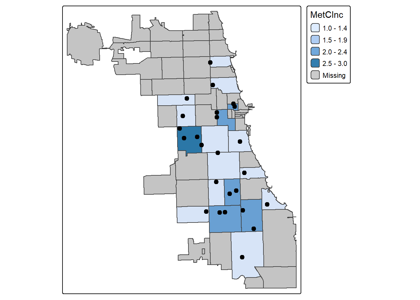
4.4 Buffer Data
Next, lets create a walkable buffer of one mile, or 5280 feet, for our MOUD provider locations. Individuals residing in places outside of that walkable area may have difficulty accessing this medication during crises, like a pandemic.
## Simple feature collection with 6 features and 8 fields
## Geometry type: POLYGON
## Dimension:     XY
## Bounding box:  xmin: 1145427 ymin: 1896014 xmax: 1179912 ymax: 1931535
## Projected CRS: NAD83 / Illinois East (ftUS)
##   X
## 1 3
## 2 4
## 3 5
## 4 6
## 5 7
## 6 8
##                                                           Name
## 1 Soft Landing Interventions/DBA Symetria Recovery of Lakeview
## 2                                        PDSSC - Chicago, Inc.
## 3                          Center for Addictive Problems, Inc.
## 4                                Family Guidance Centers, Inc.
## 5                                     A Rincon Family Services
## 6                                                            *
##                Address    City State   Zip
## 1 3934 N. Lincoln Ave. Chicago    IL 60613
## 2  2260 N. Elston Ave. Chicago    IL 60614
## 3     609 N. Wells St. Chicago    IL 60654
## 4  310 W. Chicago Ave. Chicago    IL 60654
## 5   3809 W. Grand Ave. Chicago    IL 60651
## 6  140 N. Ashland Ave. Chicago    IL 60607
##                                 fullAdd
## 1 3934 N. Lincoln Ave. Chicago IL 60613
## 2  2260 N. Elston Ave. Chicago IL 60614
## 3     609 N. Wells St. Chicago IL 60654
## 4  310 W. Chicago Ave. Chicago IL 60654
## 5   3809 W. Grand Ave. Chicago IL 60651
## 6  140 N. Ashland Ave. Chicago IL 60607
##   geo_method                       geometry
## 1     census POLYGON ((1167740 1926255, ...
## 2     census POLYGON ((1168943 1915110, ...
## 3     census POLYGON ((1179912 1904257, ...
## 4     census POLYGON ((1179283 1905671, ...
## 5     census POLYGON ((1155987 1908328, ...
## 6        osm POLYGON ((1170907 1901294, ...
Inspect immediately:
4.5 Count buffers by area
We know that MOUD locations are accessible up to one mile away. So, a total count of resources by area may be too restrictive. Let’s calculate how many walkable MOUD clinics are in each zip code. Or, how many buffers are in each area…
## [1] 2 2 1 1 1 2Stick buffer totals back to the zip master file:
## Simple feature collection with 6 features and 33 fields
## Geometry type: MULTIPOLYGON
## Dimension:     XY
## Bounding box:  xmin: 1173038 ymin: 1889918 xmax: 1183259 ymax: 1902959
## Projected CRS: NAD83 / Illinois East (ftUS)
##     zip objectid shape_area shape_len
## 1 60601       27    9166246  19804.58
## 2 60602       26    4847125  14448.17
## 3 60603       19    4560229  13672.68
## 4 60604       48    4294902  12245.81
## 5 60605       20   36301276  37973.35
## 6 60606       31    6766411  12040.44
##   Case.Rate...Cumulative year totPopE
## 1                 1451.4 2018   14675
## 2                 1688.1 2018    1244
## 3                 1107.3 2018    1174
## 4                 3964.2 2018     782
## 5                 1420.8 2018   27519
## 6                 2289.6 2018    3101
##   whiteP blackP amIndP asianP pacIsP otherP
## 1  74.17   5.57   0.45  18.00   0.00   1.81
## 2  68.17   3.78   5.31  19.45   0.00   3.30
## 3  63.46   3.24   0.00  27.60   0.00   5.71
## 4  63.43   5.63   0.00  29.67   0.00   1.28
## 5  61.20  17.18   0.18  16.10   0.03   5.31
## 6  72.75   2.35   0.00  18.09   0.00   6.80
##   hispP noHSP age0_4 age5_14 age15_19
## 1  8.68  0.00    550     156      907
## 2  6.51  0.00     61      87       18
## 3  9.80  0.00     13      43      179
## 4  4.35  0.00     12       7       52
## 5  5.84  2.39    837    1279     2172
## 6  6.29  0.73     57      44        0
##   age20_24 age15_44 age45_49 age50_54
## 1      909     8726      976     1009
## 2       91      987       46       53
## 3      172      684       75       47
## 4      168      450       27       47
## 5     2282    16364     1766     1520
## 6      139     1863      213      153
##   age55_59 age60_64 ageOv65 ageOv18
## 1      324      859    2075   13855
## 2        0        5       5    1095
## 3      150       50     112    1118
## 4       54       92      93     744
## 5     1824     1360    2569   25259
## 6      168      172     431    3000
##   age18_64 a15_24P und45P ovr65P disbP
## 1    11780   12.37  64.27  14.14   6.4
## 2     1090    8.76  91.24   0.40   0.2
## 3     1006   29.90  63.03   9.54   7.3
## 4      651   28.13  59.97  11.89   4.1
## 5    22690   16.19  67.15   9.34   5.3
## 6     2569    4.48  63.33  13.90   1.9
##   MetClnc bufferct
## 1      NA        2
## 2      NA        2
## 3      NA        1
## 4      NA        1
## 5      NA        1
## 6      NA        2
##                         geometry
## 1 MULTIPOLYGON (((1177742 190...
## 2 MULTIPOLYGON (((1181226 190...
## 3 MULTIPOLYGON (((1179499 190...
## 4 MULTIPOLYGON (((1174763 189...
## 5 MULTIPOLYGON (((1178341 189...
## 6 MULTIPOLYGON (((1174681 190...
Map density of buffers per census area:
tm_shape(areas) + tm_polygons("bufferct", fill.scale=tm_scale_intervals(values = "brewer.bu_gn", n=5, style = "jenks")) +
    tm_shape(ptbuffers) + tm_fill("gray90", fill_alpha=0.6) +
tm_shape(points) + tm_dots("gray10", size = 0.3) 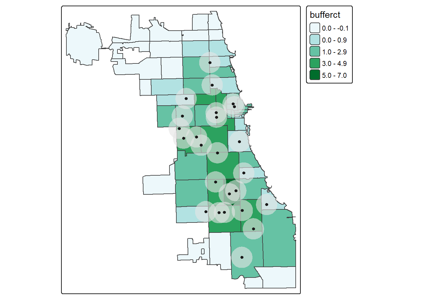
Let’s review: our master area file now has total number resources by zip and total number of walkable service areas by zip.
Using your new spatial file, see if you can answer some of these quetions using various queries:
Which zip codes have high rates of COVID and are not within a walking distance of a methadone MOUD?
Which zip codes have worse access to affordable rental units, low educational rates, and less walkable access to MOUDs?
What is the demographic and racial/ethnic characteristics of areas most vulnerable to high COVID rates in September 2020?
Generate different maps and outputs to drive your thinking and defend your hypothesis formation.
Finally, don’t forget to save your data!
Practice in Sweden
Identify a resource as a point dataset in Sweden. Then:
- Calculate count of resources per DeSo.
- Calculate a reasonable buffer distance for each resource, according to transit behavior expected.
- Calculate count of buffers per DeSo.
More Resources
Ready for the next step in calculating spatial access metrics and analying point patterns?
Nearest distance analysis: https://geodacenter.github.io/opioid-environment-toolkit/centroid-access-tutorial.html
Point pattern analyses: https://mgimond.github.io/Spatial/point-pattern-analysis-in-r.html
Rapid Realistic Routing (r5r): Routable transit metrics & travel time matrix generation: https://ipeagit.github.io/r5r/articles/r5r.html