1 Intro to Spatial Data
In the workshop, we learned about:
- What is Spatial Data?
- What is the
sfframework for R?
To delve in further, let’s see some spatial data in action.
We’ll work with the sf library first.
## Linking to GEOS 3.14.1, GDAL 3.12.1, PROJ
## 9.7.1; sf_use_s2() is TRUE1.1 Load Spatial Data
First load in the shapefile. Remember, this type of data is actually comprised of multiple files. All need to be present in order to read correctly.
## Reading layer `geo_export_aae47441-adab-4aca-8cb0-2e0c0114096e' from data source `C:\Users\wimer\github\oeps\Spatial-Health-Workshop\data\geo_export_aae47441-adab-4aca-8cb0-2e0c0114096e.shp'
## using driver `ESRI Shapefile'
## Simple feature collection with 801 features and 9 fields
## Geometry type: POLYGON
## Dimension: XY
## Bounding box: xmin: -87.94025 ymin: 41.64429 xmax: -87.52366 ymax: 42.02392
## Geodetic CRS: WGS84(DD)1.2 Non-Spatial & Spatial Views
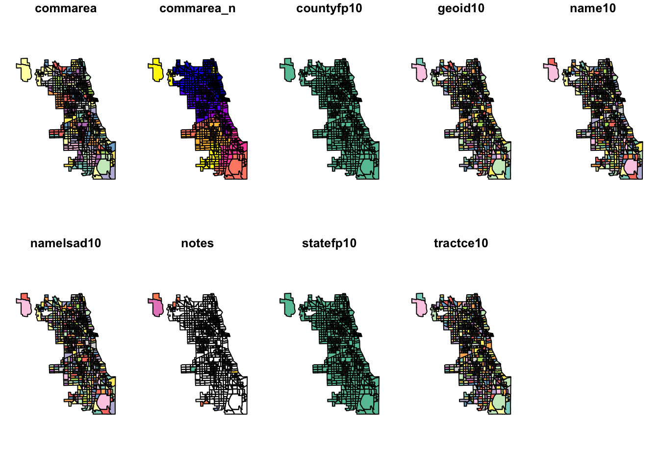
Always inspect data when loading in. First we look at a non-spatial view.
## Simple feature collection with 6 features and 9 fields
## Geometry type: POLYGON
## Dimension: XY
## Bounding box: xmin: -87.68822 ymin: 41.72902 xmax: -87.62394 ymax: 41.87455
## Geodetic CRS: WGS84(DD)
## commarea commarea_n countyfp10
## 1 44 44 031
## 2 59 59 031
## 3 34 34 031
## 4 31 31 031
## 5 32 32 031
## 6 28 28 031
## geoid10 name10 namelsad10
## 1 17031842400 8424 Census Tract 8424
## 2 17031840300 8403 Census Tract 8403
## 3 17031841100 8411 Census Tract 8411
## 4 17031841200 8412 Census Tract 8412
## 5 17031839000 8390 Census Tract 8390
## 6 17031838200 8382 Census Tract 8382
## notes statefp10 tractce10
## 1 <NA> 17 842400
## 2 <NA> 17 840300
## 3 <NA> 17 841100
## 4 <NA> 17 841200
## 5 <NA> 17 839000
## 6 <NA> 17 838200
## geometry
## 1 POLYGON ((-87.62405 41.7302...
## 2 POLYGON ((-87.68608 41.8229...
## 3 POLYGON ((-87.62935 41.8528...
## 4 POLYGON ((-87.68813 41.8556...
## 5 POLYGON ((-87.63312 41.8744...
## 6 POLYGON ((-87.66782 41.8741...Note the last column – this is a spatially enabled column. The data is no longer a shapefile but an sf object, comprised of polygons.
We can use a baseR function to view the spatial dimension. The sf framework enables previews of each attribute in our spatial file.
1.3 Spatial Data Structure
Check out the data structure of this file… What object is it?
## Classes 'sf' and 'data.frame': 801 obs. of 10 variables:
## $ commarea : chr "44" "59" "34" "31" ...
## $ commarea_n: num 44 59 34 31 32 28 65 53 76 77 ...
## $ countyfp10: chr "031" "031" "031" "031" ...
## $ geoid10 : chr "17031842400" "17031840300" "17031841100" "17031841200" ...
## $ name10 : chr "8424" "8403" "8411" "8412" ...
## $ namelsad10: chr "Census Tract 8424" "Census Tract 8403" "Census Tract 8411" "Census Tract 8412" ...
## $ notes : chr NA NA NA NA ...
## $ statefp10 : chr "17" "17" "17" "17" ...
## $ tractce10 : chr "842400" "840300" "841100" "841200" ...
## $ geometry :sfc_POLYGON of length 801; first list element: List of 1
## ..$ : num [1:243, 1:2] -87.6 -87.6 -87.6 -87.6 -87.6 ...
## ..- attr(*, "class")= chr [1:3] "XY" "POLYGON" "sfg"
## - attr(*, "sf_column")= chr "geometry"
## - attr(*, "agr")= Factor w/ 3 levels "constant","aggregate",..: NA NA NA NA NA NA NA NA NA
## ..- attr(*, "names")= chr [1:9] "commarea" "commarea_n" "countyfp10" "geoid10" ...Check out the coordinate reference system. What is it? What are the units?
## Coordinate Reference System:
## User input: WGS84(DD)
## wkt:
## GEOGCRS["WGS84(DD)",
## DATUM["WGS84",
## ELLIPSOID["WGS84",6378137,298.257223563,
## LENGTHUNIT["metre",1,
## ID["EPSG",9001]]]],
## PRIMEM["Greenwich",0,
## ANGLEUNIT["degree",0.0174532925199433]],
## CS[ellipsoidal,2],
## AXIS["longitude",east,
## ORDER[1],
## ANGLEUNIT["degree",0.0174532925199433]],
## AXIS["latitude",north,
## ORDER[2],
## ANGLEUNIT["degree",0.0174532925199433]]]1.4 Exploring Coordinate Reference Systems
Lets see how switching CRS changes our object. First we’ll try the Mollweide coordinate reference system that does a good job preserving area across the globe.
To transform our CRS, we use the st_transform function. To plot, we use baseR again but with some paremeter updates. Finally, we check out the CRS of our new object. What are the units? Any other details to note? Will this be appropriate for our spatial analysis?
Chi_tracts.moll <- st_transform(Chi_tracts, crs="ESRI:54009")
plot(st_geometry(Chi_tracts.moll), border = "gray", lwd = 2, main = "Mollweide", sub="preserves areas")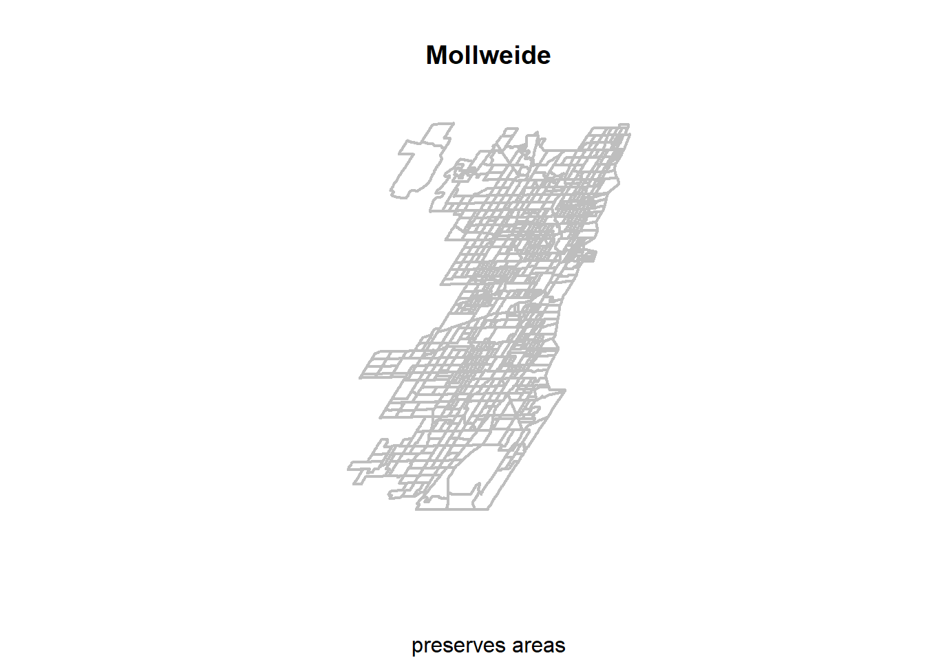
## Coordinate Reference System:
## User input: ESRI:54009
## wkt:
## PROJCRS["World_Mollweide",
## BASEGEOGCRS["WGS 84",
## DATUM["World Geodetic System 1984",
## ELLIPSOID["WGS 84",6378137,298.257223563,
## LENGTHUNIT["metre",1]]],
## PRIMEM["Greenwich",0,
## ANGLEUNIT["Degree",0.0174532925199433]]],
## CONVERSION["World_Mollweide",
## METHOD["Mollweide"],
## PARAMETER["Longitude of natural origin",0,
## ANGLEUNIT["Degree",0.0174532925199433],
## ID["EPSG",8802]],
## PARAMETER["False easting",0,
## LENGTHUNIT["metre",1],
## ID["EPSG",8806]],
## PARAMETER["False northing",0,
## LENGTHUNIT["metre",1],
## ID["EPSG",8807]]],
## CS[Cartesian,2],
## AXIS["(E)",east,
## ORDER[1],
## LENGTHUNIT["metre",1]],
## AXIS["(N)",north,
## ORDER[2],
## LENGTHUNIT["metre",1]],
## USAGE[
## SCOPE["Not known."],
## AREA["World."],
## BBOX[-90,-180,90,180]],
## ID["ESRI",54009]]Next, we’ll try the Winkel CRS, which is a compromise projection that facilitates minimal distortion for area, distance, and angles. We use the same approach, recyling the code with new inputs.
Chi_tracts.54019 = st_transform(Chi_tracts, crs="ESRI:54019")
plot(st_geometry(Chi_tracts.54019), border = "gray", lwd = 2, main = "Winkel", sub="minimal distortion")
## Coordinate Reference System:
## User input: ESRI:54019
## wkt:
## PROJCRS["World_Winkel_II",
## BASEGEOGCRS["WGS 84",
## DATUM["World Geodetic System 1984",
## ELLIPSOID["WGS 84",6378137,298.257223563,
## LENGTHUNIT["metre",1]]],
## PRIMEM["Greenwich",0,
## ANGLEUNIT["Degree",0.0174532925199433]]],
## CONVERSION["World_Winkel_II",
## METHOD["Winkel II"],
## PARAMETER["Longitude of natural origin",0,
## ANGLEUNIT["Degree",0.0174532925199433],
## ID["EPSG",8802]],
## PARAMETER["Latitude of 1st standard parallel",50.4597762521898,
## ANGLEUNIT["Degree",0.0174532925199433],
## ID["EPSG",8823]],
## PARAMETER["False easting",0,
## LENGTHUNIT["metre",1],
## ID["EPSG",8806]],
## PARAMETER["False northing",0,
## LENGTHUNIT["metre",1],
## ID["EPSG",8807]]],
## CS[Cartesian,2],
## AXIS["(E)",east,
## ORDER[1],
## LENGTHUNIT["metre",1]],
## AXIS["(N)",north,
## ORDER[2],
## LENGTHUNIT["metre",1]],
## USAGE[
## SCOPE["Not known."],
## AREA["World."],
## BBOX[-90,-180,90,180]],
## ID["ESRI",54019]]We could also try a totally different projection, to see how that changes our spatial object. Let’s use the “Old Hawaiian UTM Zone 4n” projection, with the EPSG identified from an online search. How does this fare?
Chi_tracts.Hawaii = st_transform(Chi_tracts, crs="ESRI:102114")
plot(st_geometry(Chi_tracts.Hawaii), border = "gray", lwd = 2, main = "Old Hawaiian UTM Zone 4N", sub="wrong projection!")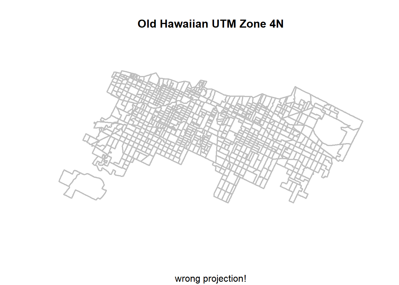
Finally.. let’s choose a projection that is focused on Illinois, and uses distance as feet or meters, to make it a bit more accessible for our work. EPSG:3435 is a good fit:
Chi_tracts.3435 <- st_transform(Chi_tracts, "EPSG:3435")
# Chi_tracts.3435 <- st_transform(Chi_tracts, 3435)
st_crs(Chi_tracts.3435)## Coordinate Reference System:
## User input: EPSG:3435
## wkt:
## PROJCRS["NAD83 / Illinois East (ftUS)",
## BASEGEOGCRS["NAD83",
## DATUM["North American Datum 1983",
## ELLIPSOID["GRS 1980",6378137,298.257222101,
## LENGTHUNIT["metre",1]]],
## PRIMEM["Greenwich",0,
## ANGLEUNIT["degree",0.0174532925199433]],
## ID["EPSG",4269]],
## CONVERSION["SPCS83 Illinois East zone (US survey foot)",
## METHOD["Transverse Mercator",
## ID["EPSG",9807]],
## PARAMETER["Latitude of natural origin",36.6666666666667,
## ANGLEUNIT["degree",0.0174532925199433],
## ID["EPSG",8801]],
## PARAMETER["Longitude of natural origin",-88.3333333333333,
## ANGLEUNIT["degree",0.0174532925199433],
## ID["EPSG",8802]],
## PARAMETER["Scale factor at natural origin",0.999975,
## SCALEUNIT["unity",1],
## ID["EPSG",8805]],
## PARAMETER["False easting",984250,
## LENGTHUNIT["US survey foot",0.304800609601219],
## ID["EPSG",8806]],
## PARAMETER["False northing",0,
## LENGTHUNIT["US survey foot",0.304800609601219],
## ID["EPSG",8807]]],
## CS[Cartesian,2],
## AXIS["easting (X)",east,
## ORDER[1],
## LENGTHUNIT["US survey foot",0.304800609601219]],
## AXIS["northing (Y)",north,
## ORDER[2],
## LENGTHUNIT["US survey foot",0.304800609601219]],
## USAGE[
## SCOPE["Engineering survey, topographic mapping."],
## AREA["United States (USA) - Illinois - counties of Boone; Champaign; Clark; Clay; Coles; Cook; Crawford; Cumberland; De Kalb; De Witt; Douglas; Du Page; Edgar; Edwards; Effingham; Fayette; Ford; Franklin; Gallatin; Grundy; Hamilton; Hardin; Iroquois; Jasper; Jefferson; Johnson; Kane; Kankakee; Kendall; La Salle; Lake; Lawrence; Livingston; Macon; Marion; Massac; McHenry; McLean; Moultrie; Piatt; Pope; Richland; Saline; Shelby; Vermilion; Wabash; Wayne; White; Will; Williamson."],
## BBOX[37.06,-89.27,42.5,-87.02]],
## ID["EPSG",3435]]plot(st_geometry(Chi_tracts.3435), border = "gray", lwd = 2, main = "NAD83 / Illinois East (ftUS)", sub="topo mapping & survey use")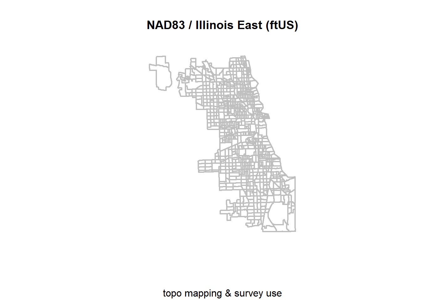
1.5 Refine Basic Map
Now we’ll switch to a more extensive cartographic mapping package, tmap. We approach mapping with one layer at a time. Always start with the object you want to map by calling it with the tm_shape function. Then, at least one descriptive/styling function follows. There are hundreds of variations and paramater specifications, so take your time in exploring tmap and the options.
Here we style the tracts with some semi-transparent borders.
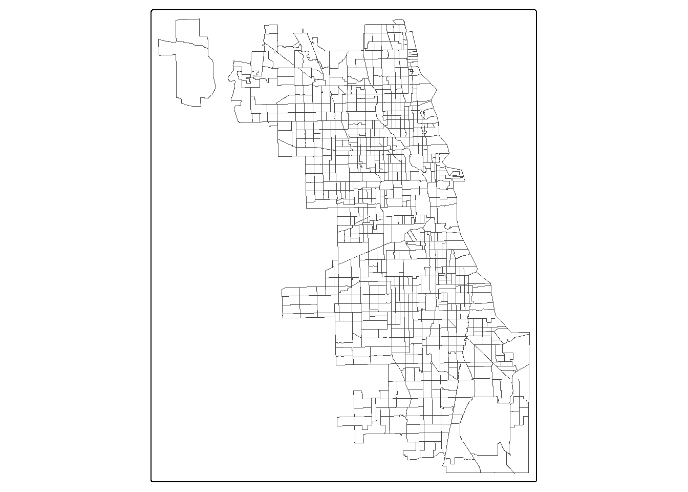
Next we fill the tracts with a light gray, and adjust the color and transparency of borders. We also add a scale bar, positioning it to the left and having a thickness of 0.8 units, and turn off the frame. See more specifications for ‘tm_polygons’ at tmap documentations.
tm_shape(Chi_tracts) +
tm_polygons(
fill = "gray90", #fill color
col = "gray10", #border color
lwd = 0.5 #line width
) +
tm_scalebar(position = c("bottom","left"), lwd = 0.8) +
tm_layout(frame = FALSE)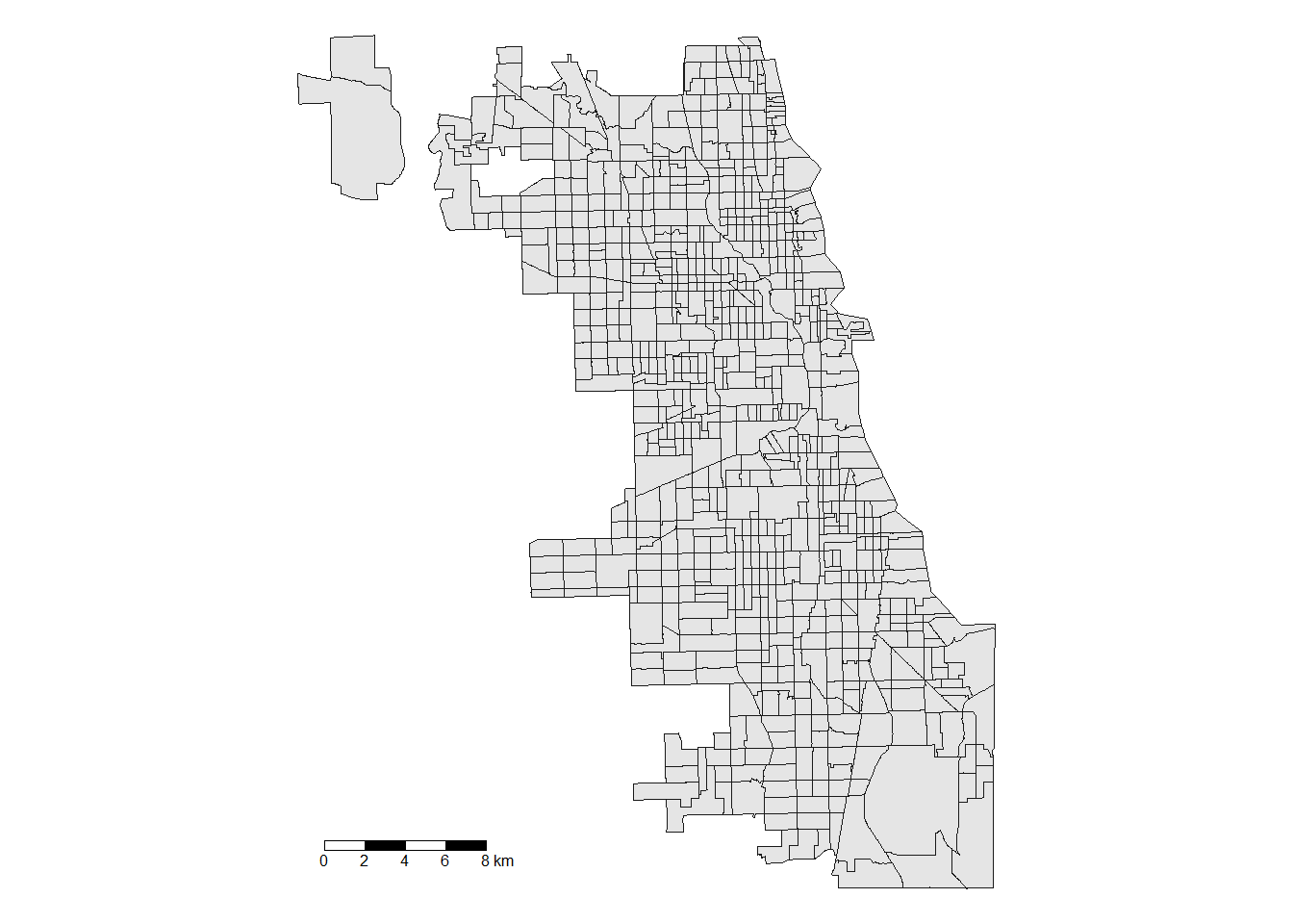
Check out the tmap Reference manual for more ideas!
1.6 Arrange multiple maps
Sometimes we want to look at multiple maps at once. Write your mapping function to a new variable, and then call that variable in order of desire using the tmap_arrange function. Hint: this is just one of many! ways to map multiples using tmap… see if you can uncover more in the documentation.
tracts.4326 <- tm_shape(Chi_tracts) +
tm_fill(col = "gray90") +
tm_title("EPSG 4326") +
tm_layout(frame = FALSE)
tracts.54019 <- tm_shape(Chi_tracts.54019) +
tm_fill(col = "gray90") +
tm_title("EPSG 54019")
tm_layout(frame = FALSE)## [nothing to show] no data layers defined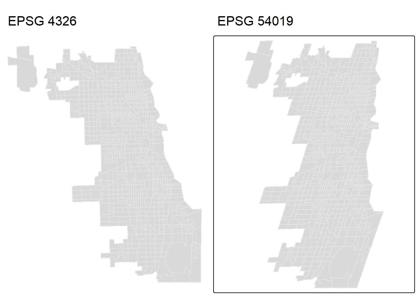
1.7 Interactive Mode
So far, we’ve been plotting static maps. We can also switch to an interactive map that uses a Leaflet widget by switching the tmap_mode() parameter specification from “plot” to “view.” It’s on “plot” as default.
## ℹ tmap modes "plot" - "view"
## ℹ toggle with `tmap::ttm()`Map the same map as before, and check out the interaction!
tm_shape(Chi_tracts) +
tm_polygons(
fill = "gray90", #fill color
col = "gray10", #border color
lwd = 0.5 #line width
) +
tm_scalebar(position = ("left"), lwd = 0.8)The tracts are not thin enough, so we update that here. We also make the fill more transparent using the ‘alpha’ parameter. You can also click the box on the left side to try out other basemaps. See if you can find out how to add a basemap to a static/plotted map, using tmap documentation…
tm_shape(Chi_tracts) +
tm_polygons(
fill = "gray90", #fill color
fill_alpha = 0.5, #fill transparency
col = "gray10", #border color
lwd = 0.25 #line width
)We revert back to plot mode for now.
## ℹ tmap modes "plot" - "view"1.8 Overlay Zip Code Boundaries
How do census tract areas correspond to zip codes? While tracts better represent neighborhoods, often times we are stuck with zip code level scale in healh research. Here we’ll make a reference map to highlight tract distribution across each zip code.
First, we read in zip code boundaries. This data was downloaded directly from the City of Chicago Data Portal as a shapefile.
## Reading layer `chicago_zips1' from data source `C:\Users\wimer\github\oeps\Spatial-Health-Workshop\data\chicago_zips1.shp'
## using driver `ESRI Shapefile'
## Simple feature collection with 59 features and 4 fields
## Geometry type: MULTIPOLYGON
## Dimension: XY
## Bounding box: xmin: -87.94011 ymin: 41.64454 xmax: -87.52414 ymax: 42.02304
## Geodetic CRS: +proj=longlat +ellps=WGS84 +no_defsNext, we layer the new shape in – on top of the tracts. We use a thicker border, and try out a new color. Experiment!
## FIRST LAYER: CENSUS TRACT BOUNADRIES
tm_shape(Chi_tracts.3435) +
tm_polygons(
fill = "gray90", #fill color
col = "gray10", #border color
lwd = 0.1 #line width
) +
## SECOND LAYER: ZIP CODE BOUNDARIES WITH LABEL
tm_shape(Chi_Zips) +
tm_borders(lwd = 2, col = "#0099CC") +
tm_text("zip", size = 0.4) +
## MORE CARTOGRAPHIC STYLE
tm_scalebar(position = c("bottom","left"), lwd = 0.8) +
tm_layout(frame = FALSE)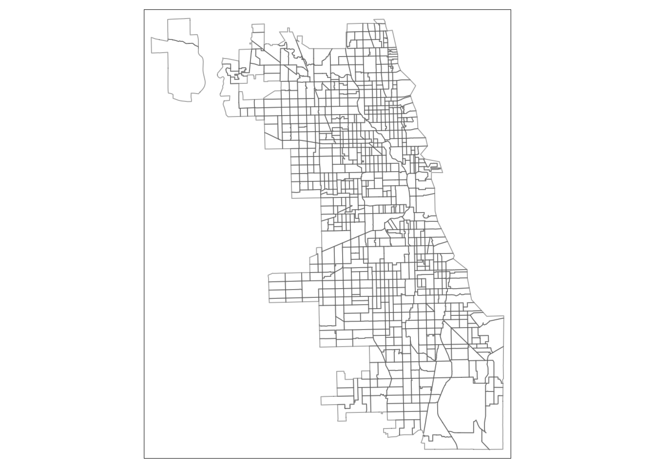
Practice in Sweden
Now practice with a new dataset! Download the DeSo file for Sweden at their official site. Scroll down to the bottom of the page, and click on “2018” for the year of reference. You can also use the file stored in this manual.
1.8.1 Open Data
Open the dataset. It is a different spatial data format, called a geopackage, but will be understood by sf as long as you include the extension in your call.
Hint
deso <- st_read("data/DeSO_2018.gpkg")
## Reading layer `DeSO_2018' from data source
## `C:\Users\wimer\github\oeps\Spatial-Health-Workshop\data\DeSO_2018.gpkg'
## using driver `GPKG'
## Simple feature collection with 5984 features and 8 fields
## Geometry type: POLYGON
## Dimension: XY
## Bounding box: xmin: 266646.3 ymin: 6132476 xmax: 920877.4 ymax: 7671055
## Projected CRS: SWEREF99 TM1.8.2 Inspect Data
Inspect the data attributes. Map the data using a simple tmap function. Ensure the data is what you expected it to be across both dimensions.
Hint
head(deso)
tm_shape(deso) + tm_polygons(fill = 'gray70', col = 'white', lwd=0.3)
## Simple feature collection with 6 features and 8 fields
## Geometry type: POLYGON
## Dimension: XY
## Bounding box: xmin: 314985.7 ymin: 6222294 xmax: 518000.7 ymax: 6402218
## Projected CRS: SWEREF99 TM
## objectid
## 1 1
## 2 2
## 3 3
## 4 4
## 5 5
## 6 1281
## objektidentitet
## 1 8de2583c-6a92-45b5-ad41-7f40b7a90862
## 2 5d108a83-8951-4345-a942-80d6f4e2d1a3
## 3 fea0f678-ed55-4cfc-8cf9-92c0050d102c
## 4 5af0864d-40f8-4599-8aa6-636d82976db3
## 5 3fa12a3d-7b03-40be-8633-4f8951101882
## 6 d315f1e1-543c-4784-94d1-0b332839ff44
## desokod regsokod lanskod kommunkod
## 1 1256B2010 1256R005 12 1256
## 2 0760B3010 0760R001 07 0760
## 3 1082C1120 1082R001 10 1082
## 4 1292A0010 1292R016 12 1292
## 5 1081C1070 1081R007 10 1081
## 6 1480C2890 1480R134 14 1480
## kommunnamn version
## 1 Östra Göinge 2018_v2
## 2 Uppvidinge 2018_v2
## 3 Karlshamn 2018_v2
## 4 Ängelholm 2018_v2
## 5 Ronneby 2018_v2
## 6 Göteborg 2018_v2
## sp_geometry
## 1 POLYGON ((442392.5 6229549,...
## 2 POLYGON ((511578.2 6330751,...
## 3 POLYGON ((490858.7 6229360,...
## 4 POLYGON ((362874.8 6230834,...
## 5 POLYGON ((517351.8 6230866,...
## 6 POLYGON ((315673.9 6401327,...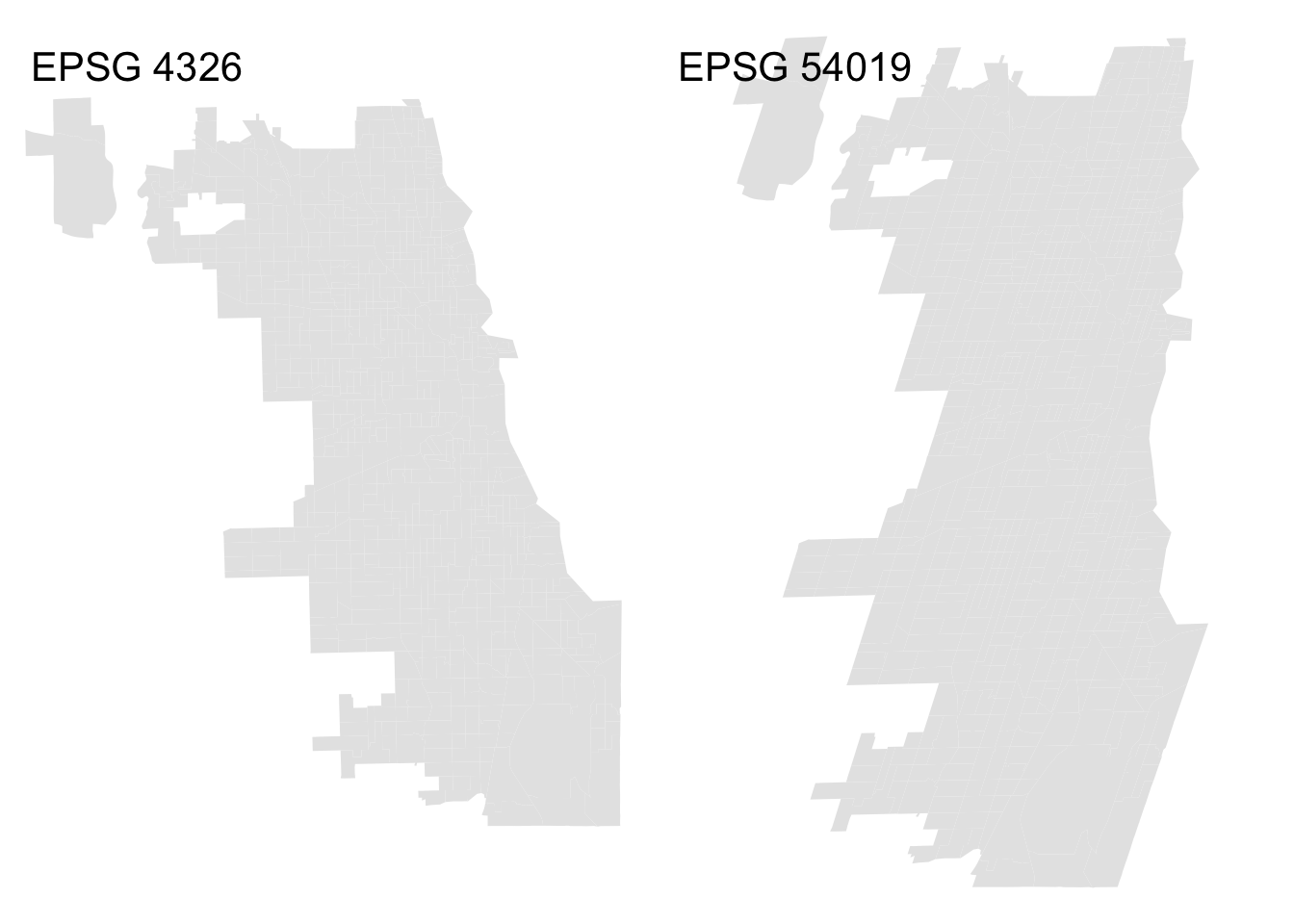
1.8.3 CRS Check
Inspect the coordinate reference system. Change the coordinate reference system to a different one.
Hint
st_crs(deso)
deso.3152 <- st_transform(deso, 3152)
## Coordinate Reference System:
## User input: SWEREF99 TM
## wkt:
## PROJCRS["SWEREF99 TM",
## BASEGEOGCRS["SWEREF99",
## DATUM["SWEREF99",
## ELLIPSOID["GRS 1980",6378137,298.257222101,
## LENGTHUNIT["metre",1]]],
## PRIMEM["Greenwich",0,
## ANGLEUNIT["degree",0.0174532925199433]],
## ID["EPSG",4619]],
## CONVERSION["SWEREF99 TM",
## METHOD["Transverse Mercator",
## ID["EPSG",9807]],
## PARAMETER["Latitude of natural origin",0,
## ANGLEUNIT["degree",0.0174532925199433],
## ID["EPSG",8801]],
## PARAMETER["Longitude of natural origin",15,
## ANGLEUNIT["degree",0.0174532925199433],
## ID["EPSG",8802]],
## PARAMETER["Scale factor at natural origin",0.9996,
## SCALEUNIT["unity",1],
## ID["EPSG",8805]],
## PARAMETER["False easting",500000,
## LENGTHUNIT["metre",1],
## ID["EPSG",8806]],
## PARAMETER["False northing",0,
## LENGTHUNIT["metre",1],
## ID["EPSG",8807]]],
## CS[Cartesian,2],
## AXIS["northing (N)",north,
## ORDER[1],
## LENGTHUNIT["metre",1]],
## AXIS["easting (E)",east,
## ORDER[2],
## LENGTHUNIT["metre",1]],
## USAGE[
## SCOPE["Topographic mapping (medium and small scale)."],
## AREA["Sweden - onshore and offshore."],
## BBOX[54.96,10.03,69.07,24.17]],
## ID["EPSG",3006]]More Resources
On spatial data basics & sf:
On projections:
On tmap: