2 Map Neighborhoods
When considering the health of persons, we have to also consider the neighborhood environment. Sometimes this is looking at neighborhood level health outcomes, like premature mortality at the census tract scale, or cumulative COVID rates by zip code. Sometimes we’re interested in neighborhood factors like poverty, access to affordable housing, or distance to nearest health provider, or pollution-emitting facility. These measurements of the “social determinants of health” at the neighborhood scale are increasingly urgent in modern public health thinking, and are thought to drive and/or reinforce racial, social, and spatial inequity
In this module, we’ll learn about the basics of thematic mapping – known as choropleth mapping – to visualize neighborhood level health phenomena. This will allow you to begin the process of exploratory spatial data analysis and hypothesis generation & refinement.
2.1 Clean Attribute Data
Let’s consider COVID-19 cases by zip code in Chicago. We’ll upload and inspect a summary of cases from the Chicago Data Portal first:
##   ZIP.Code Week.Number Week.Start
## 1    60603          39 09/20/2020
## 2    60604          39 09/20/2020
## 3    60611          16 04/12/2020
## 4    60611          15 04/05/2020
## 5    60615          11 03/08/2020
## 6    60603          10 03/01/2020
##     Week.End Cases...Weekly
## 1 09/26/2020              0
## 2 09/26/2020              0
## 3 04/18/2020              8
## 4 04/11/2020              7
## 5 03/14/2020             NA
## 6 03/07/2020             NA
##   Cases...Cumulative Case.Rate...Weekly
## 1                 13                  0
## 2                 31                  0
## 3                 72                 25
## 4                 64                 22
## 5                 NA                 NA
## 6                 NA                 NA
##   Case.Rate...Cumulative Tests...Weekly
## 1                 1107.3             25
## 2                 3964.2             12
## 3                  222.0            101
## 4                  197.4             59
## 5                     NA              6
## 6                     NA              0
##   Tests...Cumulative Test.Rate...Weekly
## 1                327               2130
## 2                339               1534
## 3                450                312
## 4                349                182
## 5                  9                 14
## 6                  0                  0
##   Test.Rate...Cumulative
## 1                27853.5
## 2                43350.4
## 3                 1387.8
## 4                 1076.3
## 5                   21.7
## 6                    0.0
##   Percent.Tested.Positive...Weekly
## 1                              0.0
## 2                              0.0
## 3                              0.1
## 4                              0.1
## 5                               NA
## 6                               NA
##   Percent.Tested.Positive...Cumulative
## 1                                  0.0
## 2                                  0.1
## 3                                  0.2
## 4                                  0.2
## 5                                   NA
## 6                                   NA
##   Deaths...Weekly Deaths...Cumulative
## 1               0                   0
## 2               0                   0
## 3               0                   0
## 4               0                   0
## 5               0                   0
## 6               0                   0
##   Death.Rate...Weekly
## 1                   0
## 2                   0
## 3                   0
## 4                   0
## 5                   0
## 6                   0
##   Death.Rate...Cumulative Population
## 1                       0       1174
## 2                       0        782
## 3                       0      32426
## 4                       0      32426
## 5                       0      41563
## 6                       0       1174
##     Row.ID            ZIP.Code.Location
## 1 60603-39 POINT (-87.625473 41.880112)
## 2 60604-39 POINT (-87.629029 41.878153)
## 3 60611-16 POINT (-87.620291 41.894734)
## 4 60611-15 POINT (-87.620291 41.894734)
## 5 60615-11 POINT (-87.602725 41.801993)
## 6 60603-10 POINT (-87.625473 41.880112)
Each row corresponds to a zip code at a different week. This data thus exists as a “long” format, which doesn’t work for spatial analysis. We need to convert to “wide” format, or at the very least, ensure that each zip code corresponds to one row.
To simplify, let’s identify the last week of the dataset, and then subset the data frame to only show that week. We will be interested in the cumulative case rate. Following is one way of doing this – can you think of another way? Try out different approaches of reshaping data to test your R and “tidy” skills.
## [1] 10 40## ZIP.Code Week.Number Week.Start
## 1 60603 39 09/20/2020
## 2 60604 39 09/20/2020
## 36 60601 39 09/20/2020
## 37 60602 39 09/20/2020
## 41 60605 39 09/20/2020
## 66 60610 39 09/20/2020
## Week.End Cases...Weekly
## 1 09/26/2020 0
## 2 09/26/2020 0
## 36 09/26/2020 8
## 37 09/26/2020 0
## 41 09/26/2020 12
## 66 09/26/2020 35
## Cases...Cumulative Case.Rate...Weekly
## 1 13 0
## 2 31 0
## 36 213 54
## 37 21 0
## 41 391 44
## 66 666 90
## Case.Rate...Cumulative Tests...Weekly
## 1 1107.3 25
## 2 3964.2 12
## 36 1451.4 202
## 37 1688.1 27
## 41 1420.8 291
## 66 1706.9 500
## Tests...Cumulative Test.Rate...Weekly
## 1 327 2130
## 2 339 1534
## 36 4304 1376
## 37 460 2170
## 41 7160 1058
## 66 10680 1281
## Test.Rate...Cumulative
## 1 27853.5
## 2 43350.4
## 36 29328.8
## 37 36977.5
## 41 26018.4
## 66 27371.3
## Percent.Tested.Positive...Weekly
## 1 0.0
## 2 0.0
## 36 0.0
## 37 0.0
## 41 0.0
## 66 0.1
## Percent.Tested.Positive...Cumulative
## 1 0.0
## 2 0.1
## 36 0.0
## 37 0.0
## 41 0.1
## 66 0.1
## Deaths...Weekly Deaths...Cumulative
## 1 0 0
## 2 0 0
## 36 1 6
## 37 0 0
## 41 1 3
## 66 0 10
## Death.Rate...Weekly
## 1 0.0
## 2 0.0
## 36 6.8
## 37 0.0
## 41 3.6
## 66 0.0
## Death.Rate...Cumulative Population
## 1 0.0 1174
## 2 0.0 782
## 36 40.9 14675
## 37 0.0 1244
## 41 10.9 27519
## 66 25.6 39019
## Row.ID ZIP.Code.Location
## 1 60603-39 POINT (-87.625473 41.880112)
## 2 60604-39 POINT (-87.629029 41.878153)
## 36 60601-39 POINT (-87.622844 41.886262)
## 37 60602-39 POINT (-87.628309 41.883136)
## 41 60605-39 POINT (-87.623449 41.867824)
## 66 60610-39 POINT (-87.63581 41.90455)To clean our data a bit, we’ll just keep the zip code name, and cumulative case rate for the week of September 20th, 2020.
##    ZIP.Code Case.Rate...Cumulative
## 1     60603                 1107.3
## 2     60604                 3964.2
## 36    60601                 1451.4
## 37    60602                 1688.1
## 41    60605                 1420.8
## 66    60610                 1706.9
2.2 Merge Spatial Data
Next, let’s merge this data to our zip code master spatial file. Reload if necessary:
## Reading layer `chicago_zips1' from data source `C:\Users\wimer\github\oeps\Spatial-Health-Workshop\data\chicago_zips1.shp'
##   using driver `ESRI Shapefile'
## Simple feature collection with 59 features and 4 fields
## Geometry type: MULTIPOLYGON
## Dimension:     XY
## Bounding box:  xmin: -87.94011 ymin: 41.64454 xmax: -87.52414 ymax: 42.02304
## Geodetic CRS: +proj=longlat +ellps=WGS84 +no_defs## Simple feature collection with 6 features and 4 fields
## Geometry type: MULTIPOLYGON
## Dimension: XY
## Bounding box: xmin: -87.80649 ymin: 41.88747 xmax: -87.59852 ymax: 41.93228
## Geodetic CRS: +proj=longlat +ellps=WGS84 +no_defs
## objectid shape_area shape_len zip
## 1 33 106052287 42720.04 60647
## 2 34 127476051 48103.78 60639
## 3 35 45069038 27288.61 60707
## 4 36 70853834 42527.99 60622
## 5 37 99039621 47970.14 60651
## 6 38 23506056 34689.35 60611
## geometry
## 1 MULTIPOLYGON (((-87.67762 4...
## 2 MULTIPOLYGON (((-87.72683 4...
## 3 MULTIPOLYGON (((-87.785 41....
## 4 MULTIPOLYGON (((-87.66707 4...
## 5 MULTIPOLYGON (((-87.70656 4...
## 6 MULTIPOLYGON (((-87.61401 4...Next, merge on zip code ID. The key in the Chi_Zips object is zip, whereas the key for the COVID data is ZIP.code. Always merge non-spatial to spatial data, not the other way around. Think of the spatial file as your master file that you will continue to add on to…
Chi_Zipsf <- merge(Chi_Zips, COVID.39f, by.x = "zip", by.y = "ZIP.Code", all = TRUE)

head(Chi_Zipsf)
## Simple feature collection with 6 features and 5 fields
## Geometry type: MULTIPOLYGON
## Dimension: XY
## Bounding box: xmin: -87.63999 ymin: 41.85317 xmax: -87.60246 ymax: 41.88913
## Geodetic CRS: +proj=longlat +ellps=WGS84 +no_defs
## zip objectid shape_area shape_len
## 1 60601 27 9166246 19804.58
## 2 60602 26 4847125 14448.17
## 3 60603 19 4560229 13672.68
## 4 60604 48 4294902 12245.81
## 5 60605 20 36301276 37973.35
## 6 60606 31 6766411 12040.44
## Case.Rate...Cumulative
## 1 1451.4
## 2 1688.1
## 3 1107.3
## 4 3964.2
## 5 1420.8
## 6 2289.6
## geometry
## 1 MULTIPOLYGON (((-87.62271 4...
## 2 MULTIPOLYGON (((-87.60997 4...
## 3 MULTIPOLYGON (((-87.61633 4...
## 4 MULTIPOLYGON (((-87.63376 4...
## 5 MULTIPOLYGON (((-87.62064 4...
## 6 MULTIPOLYGON (((-87.63397 4...2.3 Quantile Maps
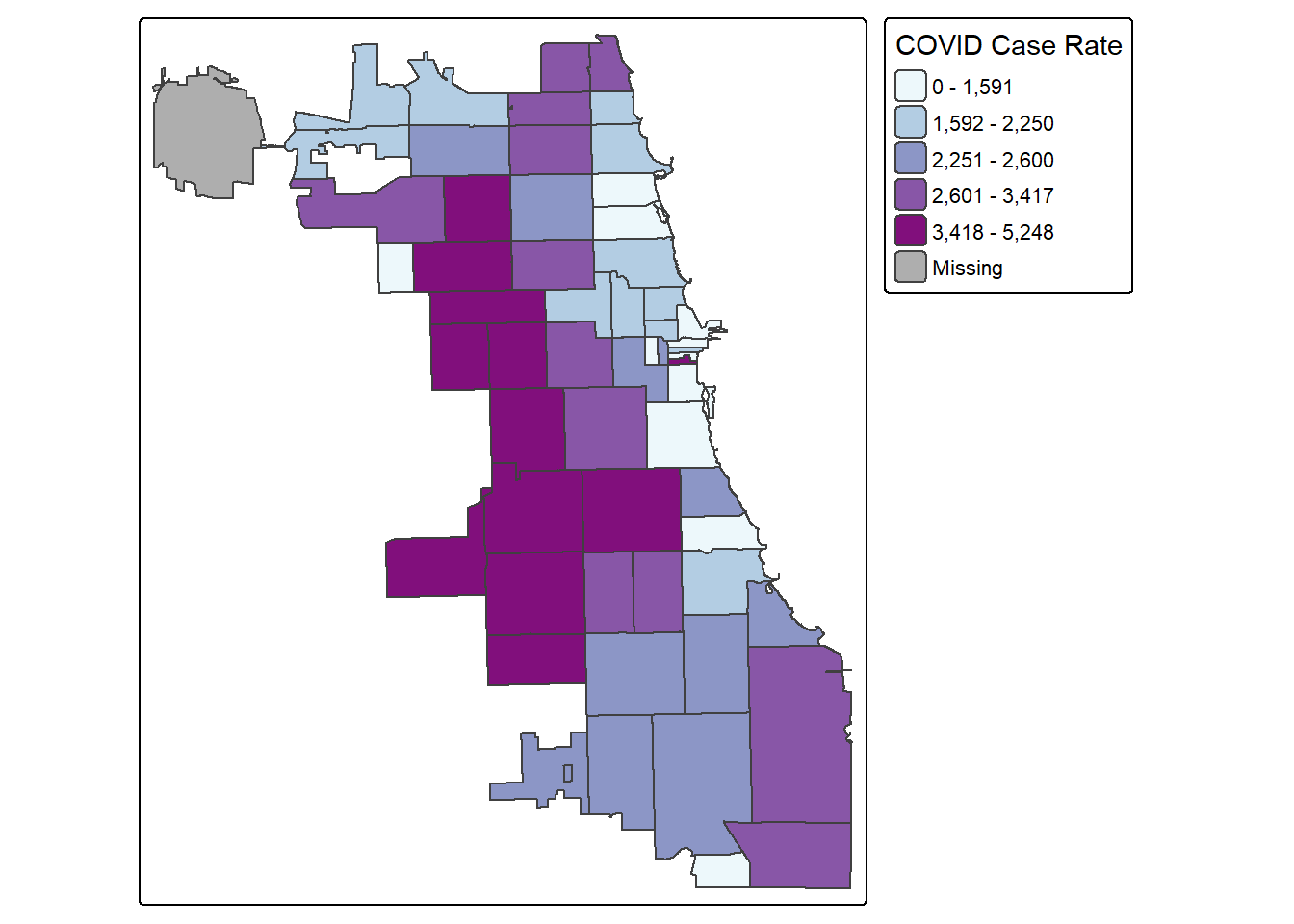
Starting with a “classic epi” approach, let’s look at case rates as quantiles. We use the tmap library, and update the choropleth data classification using the style parameter. We use the Blue-Purple palette, or BuPu, from Colorbrewer.
Colorbrewer Tip: To display all Colorbrewer palette options, load the RColorBrewer library and run display.brewer.all() – or just Google “R Colorbrewer palettes.”
library(tmap)

tmap_mode("plot")

tm_shape(Chi_Zipsf) +
  tm_polygons("Case.Rate...Cumulative",
              fill.scale  = tm_scale_intervals(style="quantile",
                                               values="BuPu"),
              fill.legend = tm_legend(title="COVID Case Rate")
              )
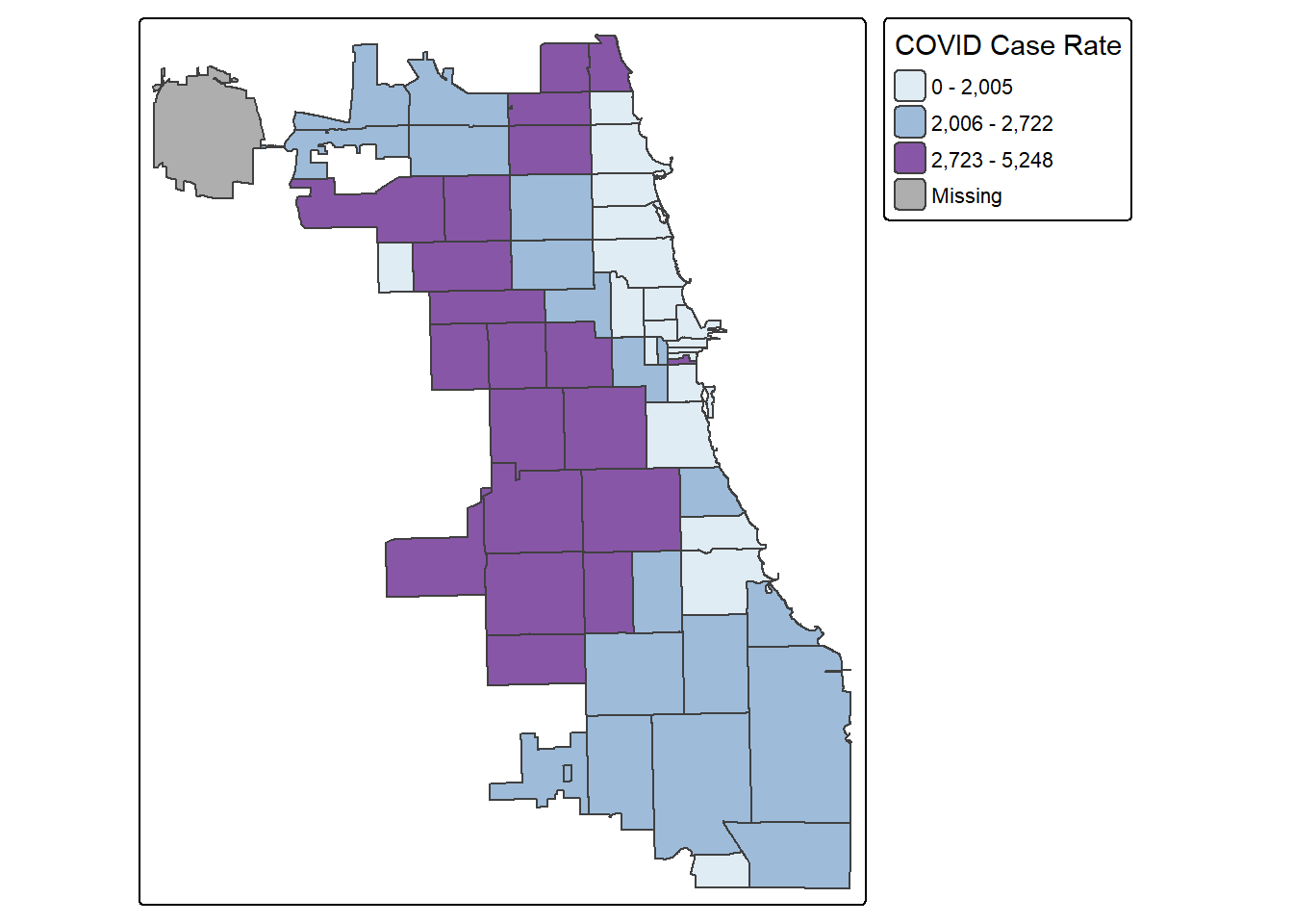
Let’s try tertiles:
tm_shape(Chi_Zipsf) +
  tm_polygons("Case.Rate...Cumulative",
              fill.scale=tm_scale_intervals(style='quantile',
                                            values="BuPu",
                                            n=3),
              fill.legend=tm_legend(title="COVID Case Rate")
              )
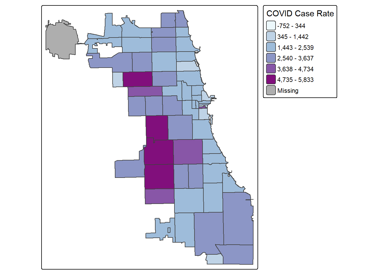
2.4 Standard Deviation Maps
While quantiles are a nice start, let’s classify using a standard deviation map. Standard deviation is a statistical technique type of map based on how much the data differs from the mean.
tm_shape(Chi_Zipsf) +
  tm_polygons("Case.Rate...Cumulative",
              fill.scale=tm_scale_intervals(style='sd',
                                            values="BuPu"),
              fill.legend=tm_legend("COVID Case Rate")
              )
2.5 Jenks Maps
Another approach of data classification is natural breaks, or jenks. This approach looks for “natural breaks” in the data using a univariate clustering algorithm.
tm_shape(Chi_Zipsf) +
  tm_polygons("Case.Rate...Cumulative",
              fill.scale=tm_scale_intervals(style="jenks",
                                            values="BuPu"),
              fill.legend=tm_legend(title="COVID Case Rate"))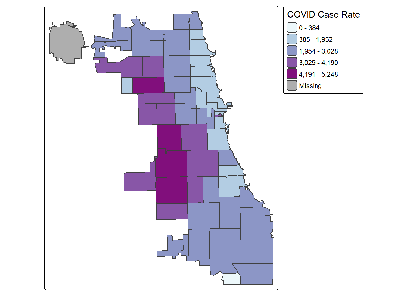
The first bin doesn’t seem very intuitive. Let’s try 4 bins instead of 5 by changing the n parameter. In this version, we’ll also had a histogram and scale bar, and move the legend outside the frame to make it easier to view.
tm_shape(Chi_Zipsf) +
  tm_polygons("Case.Rate...Cumulative",
              fill.scale=tm_scale_intervals(style="jenks",
                                            values="BuPu",
                                            n=4),
              fill.legend=tm_legend(title="COVID Case Rate")) +
  tm_scalebar(position="left")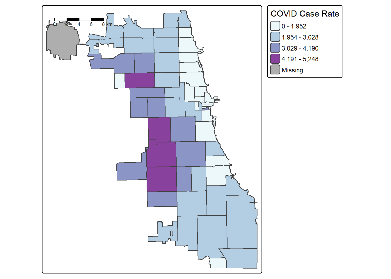
2.6 Integrate More Data
To explore potential disparities in COVID health outcomes, let’s bring in pre-cleaned demographic, racial, and ethnic data from the Opioid Environment Policy Scan database. This data is orginally sourced from the American Community Survey 2018 5-year estimate, which you could also pull using the tidycensus.
##    ZCTA year totPopE whiteP blackP amIndP
## 1 35004 2018   11762  84.39  13.09   0.00
## 2 35005 2018    7528  55.22  42.44   0.64
## 3 35006 2018    2927  96.04   3.21   0.27
## 4 35007 2018   26328  73.83  13.75   0.04
## 5 35010 2018   20625  63.07  32.43   0.39
## 6 35013 2018      40 100.00   0.00   0.00
##   asianP pacIsP otherP  hispP  noHSP age0_4
## 1   0.94   0.00   1.57   0.94   5.52    787
## 2   0.00   0.15   1.55   1.37  17.48    511
## 3   0.00   0.00   0.48   0.00  14.44    161
## 4   1.33   0.02  11.01  11.11  12.41   1891
## 5   0.65   0.00   3.45   4.10  22.00   1013
## 6   0.00   0.00   0.00 100.00 100.00      0
##   age5_14 age15_19 age20_24 age15_44
## 1    1950      457      746     4552
## 2    1055      455      277     2429
## 3     413      141      203      878
## 4    4161     1619     1400     9947
## 5    2647     1383     1087     7036
## 6       0        0        0       13
##   age45_49 age50_54 age55_59 age60_64
## 1      662      541      776      832
## 2      580      469      560      552
## 3      129      193      316      278
## 4     1993     2067     1713     1315
## 5     1418     1545     1510     1341
## 6        8       19        0        0
##   ageOv65 ageOv18 age18_64 a15_24P und45P
## 1    1662    8820     7158   10.23  61.97
## 2    1372    5691     4319    9.72  53.07
## 3     559    2308     1749   11.75  49.61
## 4    3241   19178    15937   11.47  60.77
## 5    4115   16142    12027   11.98  51.86
## 6       0      40       40    0.00  32.50
##   ovr65P disbP
## 1  14.13  12.7
## 2  18.23  23.2
## 3  19.10  20.9
## 4  12.31  13.5
## 5  19.95  19.6
## 6   0.00   0.0
Merge to our master Zip Code dataset. There are many more zip codes than we have in our Chicago dataset, so we only keep the zip codes in the main dataset, Chi_Zipf. In this case, let’s test the merge to see if we retain 61 observations.
Chi_Zips_test <- merge(Chi_Zipsf, CensusVar, by.x = "zip", by.y = "ZCTA", all.x=TRUE)

dim(Chi_Zips_test)
## [1] 60 322.7 Thematic Map Panel
To facilitate data discovery, we likely want to explore multiple maps at once. Here we’ll generate maps for multiple variables, and plot them as a map panel.
Can you think of more efficient ways to run this code? There are also other tmap tricks to optimize this further, so enjoy your journey!
Chi_Zipsf <- Chi_Zips_test

tm_shape(Chi_Zipsf) +
  tm_fill("ovr65P",
          fill.scale=tm_scale_intervals(style='jenks',
                                        values='BuPu',
                                        n=4))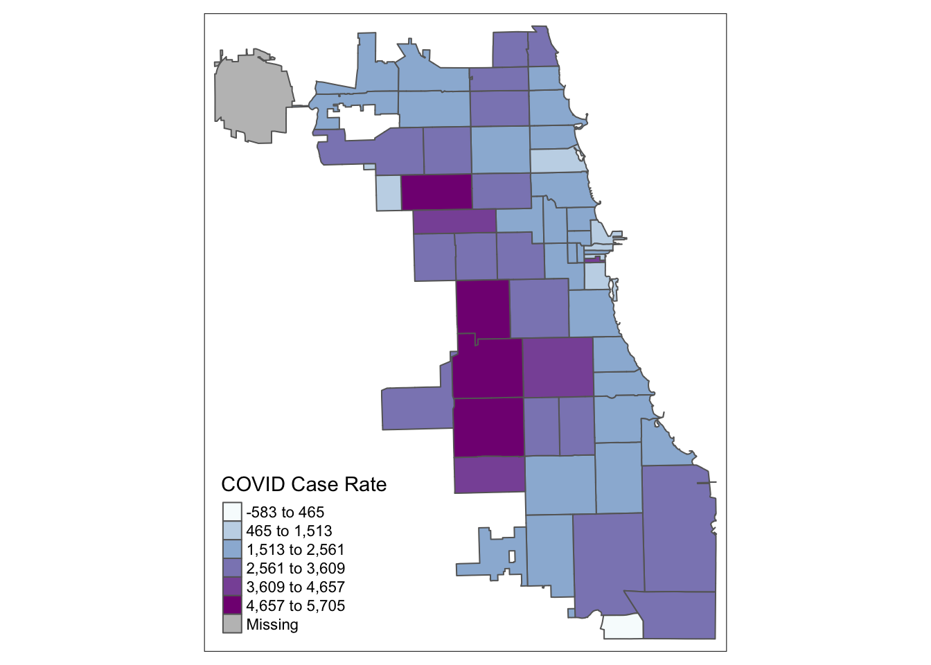
COVID <- tm_shape(Chi_Zipsf) +
  tm_fill("Case.Rate...Cumulative",
          fill.scale  = tm_scale_intervals(style='jenks', values='Reds', n=4),
          fill.legend = tm_legend("COVID Rt"))

Senior <- tm_shape(Chi_Zipsf) +
  tm_fill("ovr65P", fill.scale = tm_scale_intervals(style="jenks",
                                                   values="BuPu", n=4))

NoHS <- tm_shape(Chi_Zipsf) +
  tm_fill("noHSP", fill.scale = tm_scale_intervals(style='jenks',
                                                   values='BuPu', n=4))

BlkP <- tm_shape(Chi_Zipsf) +
  tm_fill("blackP", fill.scale = tm_scale_intervals(style='jenks',
                                                    values='BuPu', n=4))

Latnx <- tm_shape(Chi_Zipsf) +
  tm_fill("hispP", fill.scale = tm_scale_intervals(style='jenks',
                                                   values='BuPu', n=4))

WhiP <- tm_shape(Chi_Zipsf) +
  tm_fill("whiteP", fill.scale = tm_scale_intervals(style='jenks',
                                                    values='BuPu', n=4))

tmap_arrange(COVID, Senior, NoHS, BlkP, Latnx, WhiP)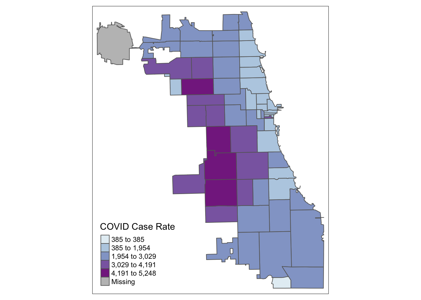
From the results, we see that cumulative COVID outcomes for one week in September 2020 seemed to have some geographic correlation with the Latinx/Hispanic community in Chicago. At the same time, low high school diploma rates are also concentrated in these areas, and there is some intersection with other variables considered. What are additional variables you could bring in to refine your approach? Perhaps percentage of essential workers; a different age group; internet access? What about linking in health outcomes like Asthma, Hypertension, and more at a similar scale?
In modern spatial epidemiology, associations must never be taken at face value. For example, we know that it is not “race” but “racism” that drives multiple health disparities – simply looking at a specific racial/ethnic group is not enough. Thus exploring multiple variables and nurturing a curiosity to understand these complex intersections will support knowledge discovery.
2.8 Data
We’re done! Well… not so fast. Let’s save the data so we don’t have to run the codebook again to access the data. Here, we’ll save as a geojson file. This spatial format is more forgiving with long column names, which is a long-standing challenge with shapefiles. But sometimes it can be written oddly, so double-check the dimensions when reading in later.
#Chi_Zipsf_recast <- st_cast(Chi_Zipsf, "MULTIPOLYGON")

#st_write(Chi_Zipsf_recast, "data/ChiZipMaster.geojson", driver = "GeoJSON")
We could also just the data as a CSV file which may be easier for future linking. For this, we use the st_drop_geometry() function to remove the geometry data, so we’re just left with the attributes.
Practice in Sweden
The data folder has a dataset entitled sweden_income_2022.csv. Bring it into the workspace. Then:
- Bring it into the workspace, and inspect. Prepare for a merge.
- Merge the income-level data to the DeSo dataset you worked with in the prior practice. Inspect.
- Generate a series of choropleth maps of median income using different styles. Select the best, and explain why you identified it as such.