Lab 5. Modeling Neighborhoods
Overview
In this practical, we will identify and quantify crimes at a local areal level for two major cities using data from open data portals. This week’s objectives will be to:
- wrangle and clean raw crime data in R
- convert CSV to spatial points for analysis & visualization
- enable and transform Coordinate Reference Systems (CRS)
- spatially join points to tracts (‘point in polygon’ analysis)
Research Question
This lab practical reflects work done in an actual research study. A team of clinicians, epidemiologists, and other health researchers were interested in comparing differences in access to trauma hospitals across three major cities. Victims of violent crime need quick access to trauma hospitals to ensure optimal results; if areas with disprortionately high homicides are especially far from trauma ERs, health outcomes can be disproportionately worse. The goal of this practical is to generate a new spatial variable, total number of homicides per census tract, in two major cities (LA and NYC) using raw data from each city’s data portal, for further analysis. Homicides were used to proxy violent crime because differenes in reporting structures on violent crime were too different for effective comparison otherwise.
You can read more about the study at: Tung, E. L., Hampton, D. A., Kolak, M., Rogers, S. O., Yang, J. P., & Peek, M. E. (2019). Race/Ethnicity and Geographic Access to Urban Trauma Care. JAMA network open, 2(3), e190138-e190138..
Environment Setup
For this lab, you’ll need to have R and RStudio downloaded and installed on your system. We will work with the following libraries, so please be sure to have already installed:
- sf
- tmap
- leaflet
- data.table
- tidyverse
First, load the libraries we’ll need for our lab.
## Linking to GEOS 3.7.2, GDAL 2.4.2, PROJ 5.2.0## ── Attaching packages ──────────────── tidyverse 1.3.0 ──## ✓ ggplot2 3.3.0 ✓ purrr 0.3.4
## ✓ tibble 3.0.1 ✓ dplyr 0.8.5
## ✓ tidyr 1.0.3 ✓ stringr 1.4.0
## ✓ readr 1.3.1 ✓ forcats 0.5.0## ── Conflicts ─────────────────── tidyverse_conflicts() ──
## x dplyr::between() masks data.table::between()
## x dplyr::filter() masks stats::filter()
## x dplyr::first() masks data.table::first()
## x dplyr::lag() masks stats::lag()
## x dplyr::last() masks data.table::last()
## x purrr::transpose() masks data.table::transpose()Set your working directory.
#setwd("~/Desktop/Lab5-LACrimes")Clean & Wrangle Data
We will be working with crime data from the Los Angeles open data portal first. When working with crime data, we will filter to the year of interest within the data portal, and then download the filtered dataset. This is because downloading all crimes produces an unnecessarily large dataset, from which we just need a short period of data. Unless you are interested in all crimes across time, start with a smaller subset that is more closely matched to your period of interest. As you get more comfortable with coding and optimizing speed and efficiency, your process may change.
In this lab practical, all violent crimes from 2015 are provided as the filtered, downloaded dataset that we start with. From these violent crimes, we are tasked with identifying “homicides” to make more comparable variables between cities. We must identify rows coded as homicides in LA, and will later do the same for NYC. Note that each police department jurisdiction codes slightly differently. Identifying data for true and meaningful comparison is an important step in the research process.
Load CSV with fread
Load the filtered CSV of crimes in Los Angeles from 2015. Here we use the fread function from the data.table package, which reads in CSV data much more quickly and efficiently then the base R system.
LAcrime<-fread("LAPD2015_Violent.csv", header = T)
head(LAcrime)
## DR Number Date Reported Date Occurred Time Occurred Area ID Area Name
## 1: 151504287 1/5/15 1/5/15 1320 15 N Hollywood
## 2: 151504288 1/5/15 1/5/15 1320 15 N Hollywood
## 3: 151504289 1/5/15 1/5/15 1320 15 N Hollywood
## 4: 151504298 1/6/15 1/5/15 1140 15 N Hollywood
## 5: 150104246 1/6/15 1/6/15 600 1 Central
## 6: 151704164 1/6/15 1/6/15 520 17 Devonshire
## Reporting District Crime Code Crime Code Description
## 1: 1599 231 ASSAULT WITH DEADLY WEAPON ON POLICE OFFICER
## 2: 1599 231 ASSAULT WITH DEADLY WEAPON ON POLICE OFFICER
## 3: 1599 231 ASSAULT WITH DEADLY WEAPON ON POLICE OFFICER
## 4: 1599 231 ASSAULT WITH DEADLY WEAPON ON POLICE OFFICER
## 5: 152 231 ASSAULT WITH DEADLY WEAPON ON POLICE OFFICER
## 6: 1785 231 ASSAULT WITH DEADLY WEAPON ON POLICE OFFICER
## MO Codes Victim Age Victim Sex Victim Descent Premise Code
## 1: 1212 1100 NA M B 501
## 2: 1212 NA M O 501
## 3: 1212 NA M O 501
## 4: 1212 31 M H 710
## 5: 416 20 M H 101
## 6: 1271 1309 2003 1822 NA F H 101
## Premise Description Weapon Used Code Weapon Description
## 1: SINGLE FAMILY DWELLING 109 SEMI-AUTOMATIC PISTOL
## 2: SINGLE FAMILY DWELLING 109 SEMI-AUTOMATIC PISTOL
## 3: SINGLE FAMILY DWELLING 109 SEMI-AUTOMATIC PISTOL
## 4: OTHER PREMISE 102 HAND GUN
## 5: STREET 500 UNKNOWN WEAPON/OTHER WEAPON
## 6: STREET 307 VEHICLE
## Status Code Status Description Crime Code 1 Crime Code 2 Crime Code 3
## 1: AA Adult Arrest 231 NA NA
## 2: AA Adult Arrest 231 NA NA
## 3: AA Adult Arrest 231 NA NA
## 4: AA Adult Arrest 231 NA NA
## 5: AA Adult Arrest 231 NA NA
## 6: AA Adult Arrest 231 NA NA
## Crime Code 4 Address
## 1: NA 7700 SKYHILL DR
## 2: NA 7700 SKYHILL DR
## 3: NA 7700 SKYHILL DR
## 4: NA 7700 SKYHILL DR
## 5: NA GRAND AV
## 6: NA PRAIRIE
## Cross Street location latitude longitude
## 1: 34.133, -118.3644 34.133 -118.3644
## 2: 34.133, -118.3644 34.133 -118.3644
## 3: 34.133, -118.3644 34.133 -118.3644
## 4: 34.133, -118.3644 34.133 -118.3644
## 5: 6TH ST 34.0486, -118.2554 34.0486 -118.2554
## 6: RESEDA 34.2391, -118.5361 34.2391 -118.5361Identify unique Code
Which column stores crime information? Inspect all of them in detail. In this dataset, the “Crime Code Description” attribute field seems to include information we can explore in further detail to filter out homicides.
Identify all possible crimes in the code description field using the unique function. Where such information is contained will change depending on the city and specific dataset you’re working with.
unique(LAcrime$`Crime Code Description`)## [1] "ASSAULT WITH DEADLY WEAPON ON POLICE OFFICER"
## [2] "ASSAULT WITH DEADLY WEAPON, AGGRAVATED ASSAULT"
## [3] "ATTEMPTED ROBBERY"
## [4] "BATTERY - SIMPLE ASSAULT"
## [5] "CRIMINAL HOMICIDE"
## [6] "OTHER ASSAULT"
## [7] "ROBBERY"Subset Data
Let’s subset the data to only include homicides. First, let’s make sure our file is a proper data frame.
LAcrime.df<- as.data.frame(LAcrime)Next, we subset the data. In this base R form of subsetting, we identify all crime codes with the “Criminal Homicide” code. Note that because there are spaces in the column heading for this variable, we had to use single quotes around the column heading.
# Base R subset:
s1<-subset(LAcrime.df,LAcrime.df$`Crime Code Description`== "CRIMINAL HOMICIDE")
Here, we bind all the rows (rbind) of the subset and give it a new name. This ‘sticks’ all the rows from our subset back together as a data frame.
LAcrime.hom<-rbind(s1)Challenge: This base R approach is successful here, but there are many other ways of subsetting data in R that are more elegant (and don’t require the data frame check or rbind step). As a challenge, explore more options on your own! Hint: check filter from dplyr.
Inspect Data
Let’s preview the first six rows of the data subset, and check dimensions. How many homicides were in LA in 2015? Hint: the total number of observations = crimes.
head(s1)## DR Number Date Reported Date Occurred Time Occurred Area ID Area Name
## 29097 151015594 10/2/15 1/1/15 6 10 West Valley
## 29098 151604033 1/2/15 1/2/15 755 16 Foothill
## 29099 150200508 1/4/15 1/3/15 2045 2 Rampart
## 29100 150604256 1/4/15 1/4/15 2355 6 Hollywood
## 29101 151804154 1/5/15 1/4/15 1900 18 Southeast
## 29102 150104310 1/7/15 1/6/15 1047 1 Central
## Reporting District Crime Code Crime Code Description
## 29097 1047 110 CRIMINAL HOMICIDE
## 29098 1675 110 CRIMINAL HOMICIDE
## 29099 211 110 CRIMINAL HOMICIDE
## 29100 646 110 CRIMINAL HOMICIDE
## 29101 1821 110 CRIMINAL HOMICIDE
## 29102 165 110 CRIMINAL HOMICIDE
## MO Codes Victim Age Victim Sex Victim Descent
## 29097 24 F W
## 29098 0430 1100 1402 1414 27 F B
## 29099 1100 0430 0906 1402 28 M H
## 29100 1100 0430 53 M B
## 29101 0906 1270 0302 0334 0430 1100 1407 28 M H
## 29102 1218 0411 34 M B
## Premise Code Premise Description Weapon Used Code
## 29097 149 RIVER BED* 500
## 29098 127 TRASH CAN/TRASH DUMPSTER 106
## 29099 102 SIDEWALK 106
## 29100 101 STREET 109
## 29101 301 GAS STATION 102
## 29102 102 SIDEWALK 204
## Weapon Description Status Code Status Description Crime Code 1
## 29097 UNKNOWN WEAPON/OTHER WEAPON IC Invest Cont 110
## 29098 UNKNOWN FIREARM IC Invest Cont 110
## 29099 UNKNOWN FIREARM AA Adult Arrest 110
## 29100 SEMI-AUTOMATIC PISTOL AA Adult Arrest 110
## 29101 HAND GUN IC Invest Cont 110
## 29102 FOLDING KNIFE AA Adult Arrest 110
## Crime Code 2 Crime Code 3 Crime Code 4
## 29097 NA NA NA
## 29098 998 NA NA
## 29099 998 NA NA
## 29100 998 NA NA
## 29101 NA NA NA
## 29102 NA NA NA
## Address
## 29097 BALBOA BL
## 29098 9100 DE GARMO AV
## 29099 600 N ALEXANDRIA AV
## 29100 1600 N CAHUENGA BL
## 29101 9900 S HOOVER ST
## 29102 600 WALL ST
## Cross Street location latitude longitude
## 29097 S VICTORY BL 34.1775, -118.5088 34.1775 -118.5088
## 29098 34.2346, -118.3741 34.2346 -118.3741
## 29099 34.0813, -118.2981 34.0813 -118.2981
## 29100 34.0998, -118.3295 34.0998 -118.3295
## 29101 33.9464, -118.2869 33.9464 -118.2869
## 29102 34.0433, -118.2488 34.0433 -118.2488Save Cleaned Data
Finally, let’s write this subset to a CSV of homicide data in LA from 2015 to archive our data as we’ve wrangled it.
write.csv(LAcrime.hom,"LAcrime_hom.csv")Convert CSV to Points
While our CSV file includes location information, it is still not spatial data because the spatial dimension has not been enabled. Let’s enable it.
First, identify which long/lat fields we are using.
Identify X,Y locations
Coordinate information is stored as columns “longitude” and “latitude” (or X,Y coordinates) corresponding to:
glimpse(LAcrime.hom[,c("longitude","latitude")])## Rows: 282
## Columns: 2
## $ longitude <chr> "-118.5088", "-118.3741", "-118.2981", "-118.3295", "-118.2…
## $ latitude <chr> "34.1775", "34.2346", "34.0813", "34.0998", "33.9464", "34.…Now we convert the crimes to points using the long/lat fields, and assign the standard projection of WGS84 using the SRID code EPSG:4326 based on our “best guess” of the actual CRS.
Remember that long = x, lat = y! If you mix this up, your points will end up getting projected on the other side of the world.
Even if we want to convert to another CRS later, we must first “respect” the CRS that the long/lat data is currently in. We use the st_as_sf function from the sf package. Uncomment and run the line below.
Check long/lat structure
Let’s check the data structure of long/lat to first confirm they are numeric:
str(LAcrime.hom[,c("longitude", "latitude")])## 'data.frame': 282 obs. of 2 variables:
## $ longitude: chr "-118.5088" "-118.3741" "-118.2981" "-118.3295" ...
## $ latitude : chr "34.1775" "34.2346" "34.0813" "34.0998" ...They are character data formats – we need numeric numbers. A quick online search shows multiple ways to convert data structures in R. We will use the as.numeric function to convert these fields.
LAcrime.hom$latitude <- as.numeric(LAcrime.hom$latitude)
LAcrime.hom$longitude <- as.numeric(LAcrime.hom$longitude)
## Warning: NAs introduced by coercionWe get a new error stating that “NAs introduced by coercion.” That suggests that we have a few observations that do not have either long/lat values! These will not be included in the final analysis. Note that we can’t convert to a spatial data format unless we remove these. Uncomment and run the folllowing:
LAcrime.pts <- st_as_sf(LAcrime.hom, coords = c("longitude","latitude"), crs = 4326)## Error in st_as_sf.data.frame(LAcrime.hom, coords = c("longitude", "latitude"), : missing values in coordinates not allowedIf we run this expression as is, we get an error that “missing values in coordinates not allowed.”
ID Missing Data
Let’s see if we can identify which observation(s) is(are) faulty. We’ll use the subset() function to see which crimes have an NA value – using the is.na() function to check for null values in the long or lat fields:
LAcrime.hom.na <- subset(LAcrime.hom, is.na(LAcrime.hom[,c("longitude", "latitude")]))

glimpse(LAcrime.hom.na) #1 observations
## Rows: 1
## Columns: 28
## $ `DR Number` <int> 151716991
## $ `Date Reported` <chr> "10/4/15"
## $ `Date Occurred` <chr> "10/4/15"
## $ `Time Occurred` <int> 2100
## $ `Area ID` <int> 17
## $ `Area Name` <chr> "Devonshire"
## $ `Reporting District` <int> 1796
## $ `Crime Code` <int> 110
## $ `Crime Code Description` <chr> "CRIMINAL HOMICIDE"
## $ `MO Codes` <chr> "1309 0554 0416 1402"
## $ `Victim Age` <int> 35
## $ `Victim Sex` <chr> "M"
## $ `Victim Descent` <chr> "B"
## $ `Premise Code` <int> 101
## $ `Premise Description` <chr> "STREET"
## $ `Weapon Used Code` <int> 307
## $ `Weapon Description` <chr> "VEHICLE"
## $ `Status Code` <chr> "AA"
## $ `Status Description` <chr> "Adult Arrest"
## $ `Crime Code 1` <int> 110
## $ `Crime Code 2` <int> 998
## $ `Crime Code 3` <int> NA
## $ `Crime Code 4` <int> NA
## $ Address <chr> "16900 NAPA ST"
## $ `Cross Street` <chr> ""
## $ location <chr> "34.2267, -118.5"
## $ latitude <dbl> 34.2267
## $ longitude <dbl> NARemove NA values
In this case we have one observation that seems to have been incorrectly coded; while location information is present, the longitude value is empty. We could assign the location value, but in this case, we will be extra cautious and remove the observation. Here we just grab the long/lat fields and the unique ID.
LAcrime.hom2 <- na.omit(LAcrime.hom[,c("DR Number","longitude", "latitude")])
str(LAcrime.hom2)
## 'data.frame': 281 obs. of 3 variables:
## $ DR Number: int 151015594 151604033 150200508 150604256 151804154 150104310 151204583 150504595 151804468 151204896 ...
## $ longitude: num -119 -118 -118 -118 -118 ...
## $ latitude : num 34.2 34.2 34.1 34.1 33.9 ...
## - attr(*, "na.action")= 'omit' Named int 225
## ..- attr(*, "names")= chr "29321"We use the str() function to ensure we have 1 less observation, for a total of 281 (out of 282).
Challenge: How would you get all the variables, minus the NA’s in long/lat?
Convert & Inspect
Now we can succesffully convert the data frame into a spatial data frame.
LAcrime.pts <- st_as_sf(LAcrime.hom2, coords = c("longitude","latitude"), crs = 4326)Let’s plot our points to make sure they look like LA:
plot(LAcrime.pts)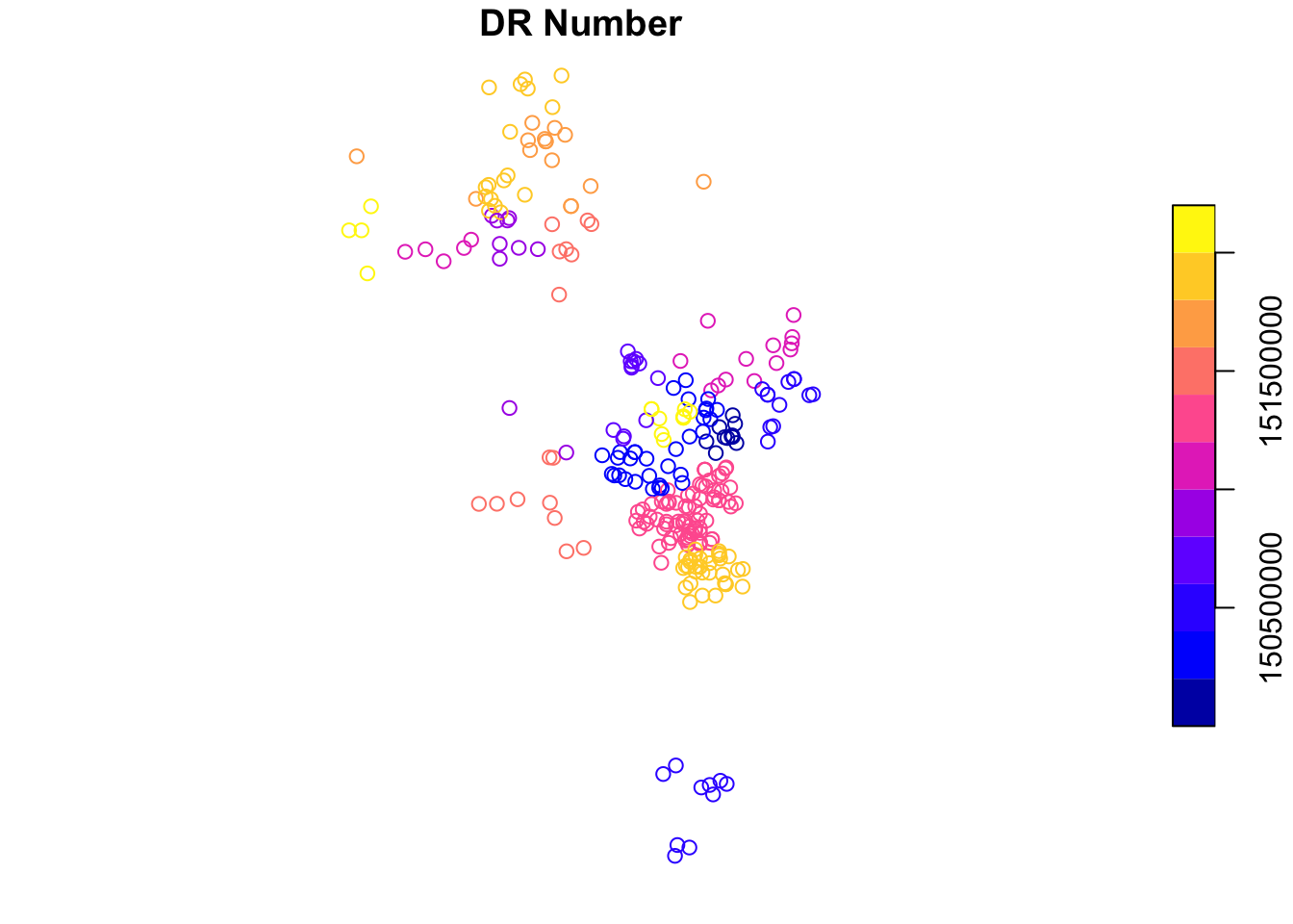
Again, if these points were not plotting correctly, you would need to check: (1) if you specified long/lat correctly or if they were flipped by accident, and (2) if the CRS you used was in fact the real CRS of the coordinates.
Save Clean Data
We now have a subset of crime data for Los Angeles in 2015 that only includes homicides, recorded as a CSV, and now as a spatial point data frame. We’ll write the homicide data with all features available to a shapefile for archiving. Uncomment and run.
#st_write(LAcrime.pts,"LAcrime_hom.shp")Rinse and Repeat
Next, do the same for the NYC dataset. What crime code description did you use? How many total homicides were there in NYC in 2015? Were there any NA values you had to deal with in the lat/long fields? Save the cleaned NYC homicide dataset as a CSV and the cleaned NYC points as a SHP.
Standardize CRS
Load & Inspect
We’ll rename the cleaned crime dataset to make it easier for analysis here. You could also load the new point shapefile you generated instead.
LAcrimes<-LAcrime.ptsNext load the LA tract shapefile, as provided in the lab materials.
LAtracts <- st_read("LAC_Shape.shp")## Reading layer `LAC_Shape' from data source `/Users/HIPark/Documents/micrometcalf/Intro2GIS/book/LAC_Shape.shp' using driver `ESRI Shapefile'
## Simple feature collection with 1009 features and 12 fields
## geometry type: POLYGON
## dimension: XY
## bbox: xmin: -118.6983 ymin: 33.69692 xmax: -118.149 ymax: 34.34164
## CRS: 4269Overlay Points & Polygons
We can plot these quickly to ensure they are overlaying correctly. If they are, our coordinate systems are working correctly.
## 1st layer (gets plotted first)
tm_shape(LAtracts) + tm_borders(alpha = 0.4) +

  ## 2nd layer (overlay)
tm_shape(LAcrime.pts) + tm_dots(size = 0.1, col="red") 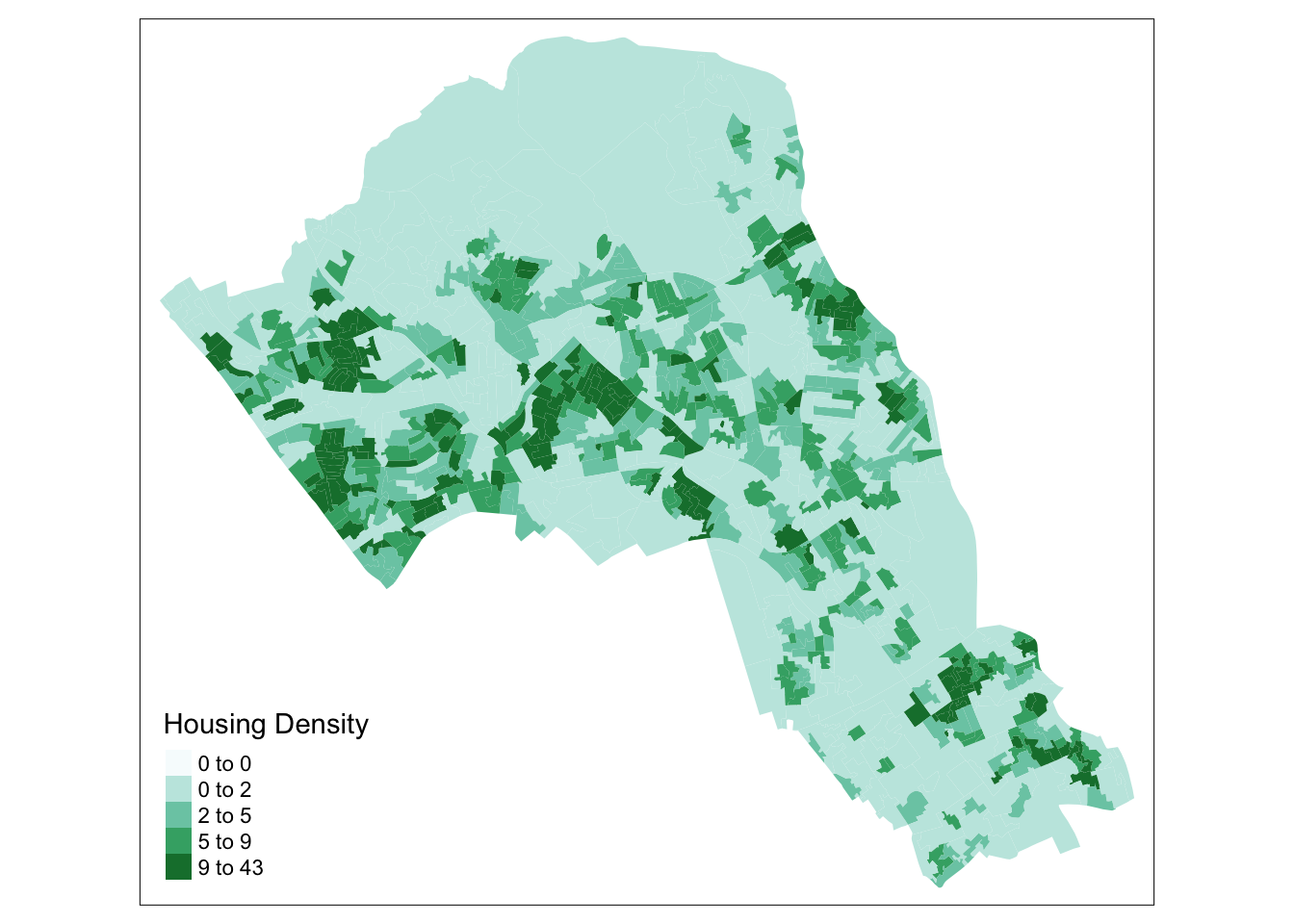
Check CRS
Check the Coordinate System/Projection for your data.
st_crs(LAcrimes) ## Coordinate Reference System:
## User input: EPSG:4326
## wkt:
## GEOGCS["WGS 84",
## DATUM["WGS_1984",
## SPHEROID["WGS 84",6378137,298.257223563,
## AUTHORITY["EPSG","7030"]],
## AUTHORITY["EPSG","6326"]],
## PRIMEM["Greenwich",0,
## AUTHORITY["EPSG","8901"]],
## UNIT["degree",0.0174532925199433,
## AUTHORITY["EPSG","9122"]],
## AUTHORITY["EPSG","4326"]]Are the coordinate systems for crime points and tracts the same?
st_crs(LAtracts)## Coordinate Reference System:
## User input: 4269
## wkt:
## GEOGCS["NAD83",
## DATUM["North_American_Datum_1983",
## SPHEROID["GRS 1980",6378137,298.257222101,
## AUTHORITY["EPSG","7019"]],
## TOWGS84[0,0,0,0,0,0,0],
## AUTHORITY["EPSG","6269"]],
## PRIMEM["Greenwich",0,
## AUTHORITY["EPSG","8901"]],
## UNIT["degree",0.0174532925199433,
## AUTHORITY["EPSG","9122"]],
## AUTHORITY["EPSG","4269"]]If they match, we are ready for point-in-polygon (PIP) or spatial join operation. R is very finicky about wanting an identical CRS specification. Since they don’t match exactly by R standards, we need to transform our files into the same projection.
Transform CRS
We’ll use the LAtracts CRS as our main projection. We then transform LAcrimes into the new projection using the st_transform function.
CRS.new <- st_crs(LAtracts)
LAcrimes <- st_transform(LAcrimes, CRS.new)
Check the CRS of both datasets again. If they are identical you’re ready to move onto the next step!
Point-in-Polygon
Our LA Crimes dataset is very small; we just kept the ID per point in case we need to merge more information from the raw data file later. We need to identify which census tract each crime occurred in, next.
glimpse(LAcrimes)## Rows: 281
## Columns: 2
## $ `DR Number` <int> 151015594, 151604033, 150200508, 150604256, 151804154, 15…
## $ geometry <POINT [°]> POINT (-118.5088 34.1775), POINT (-118.3741 34.2346…Spatial Join
First we will spatially join Crimes and Tracts. This operations uses a within operation to essentially “stick” all attributes from census tracts to the crime data file, based on the spatial location or intersection of crimes in tracts.
crime_in_tract <- st_join(LAcrimes, LAtracts, join = st_within)## although coordinates are longitude/latitude, st_within assumes that they are planarglimpse(crime_in_tract)## Rows: 281
## Columns: 14
## $ `DR Number` <int> 151015594, 151604033, 150200508, 150604256, 151804154, 15…
## $ STATEFP10 <chr> "06", "06", "06", "06", "06", "06", "06", "06", "06", "06…
## $ COUNTYFP10 <chr> "037", "037", "037", "037", "037", "037", "037", "037", "…
## $ TRACTCE10 <chr> "139001", "121102", "192610", "190700", "240402", "206300…
## $ GEOID10 <chr> "06037139001", "06037121102", "06037192610", "06037190700…
## $ NAME10 <chr> "1390.01", "1211.02", "1926.10", "1907", "2404.02", "2063…
## $ NAMELSAD10 <chr> "Census Tract 1390.01", "Census Tract 1211.02", "Census T…
## $ MTFCC10 <chr> "G5020", "G5020", "G5020", "G5020", "G5020", "G5020", "G5…
## $ FUNCSTAT10 <chr> "S", "S", "S", "S", "S", "S", "S", "S", "S", "S", "S", "S…
## $ ALAND10 <dbl> 1239788, 7458077, 415408, 642502, 601299, 616657, 742058,…
## $ AWATER10 <dbl> 0, 82268, 0, 0, 0, 0, 0, 0, 0, 0, 0, 0, 0, 0, 0, 0, 0, 0,…
## $ INTPTLAT10 <chr> "+34.1754113", "+34.2375326", "+34.0813650", "+34.0986626…
## $ INTPTLON10 <chr> "-118.5117180", "-118.3841883", "-118.2961539", "-118.333…
## $ geometry <POINT [°]> POINT (-118.5088 34.1775), POINT (-118.3741 34.2346…Note that the st_join function assumed planar coordinates, though our actual CRS is not in a planar CRS. For our purposes, because the geographic space of LA is relatively small (compared to the surface of the Earth), it will be okay. For larger areas or to be more precise, you would need to research, identify, and transform all files into a different CRS.
Count Crimes per Tract
Next, we’ll count all crimes by tract using the table function. There are many ways to do this operation in R. Inspect the output.
crime_tract_count <- as.data.frame(table(crime_in_tract$TRACTCE10))
glimpse(crime_tract_count)
## Rows: 206
## Columns: 2
## $ Var1 <fct> 101300, 104108, 104203, 104310, 104320, 104401, 104404, 104701, …
## $ Freq <int> 1, 1, 1, 1, 1, 1, 1, 2, 1, 1, 1, 1, 1, 1, 1, 1, 1, 1, 2, 1, 1, 1…As a challenge, explore more options on your own using online R resources. See if you can identify ways to do this using dyplyr functions.
Rename Column Names
We will next rename column names.
names(crime_tract_count) <- c("TRACTCE10","CrimeCt")
glimpse(crime_tract_count)
## Rows: 206
## Columns: 2
## $ TRACTCE10 <fct> 101300, 104108, 104203, 104310, 104320, 104401, 104404, 104…
## $ CrimeCt <int> 1, 1, 1, 1, 1, 1, 1, 2, 1, 1, 1, 1, 1, 1, 1, 1, 1, 1, 2, 1,…Merge Data
Now we can merge our count table back to our master LAtracts spatial file. We will use the common key “TRACTCSE10” to merge these. Inspect.
LAtracts_new <- merge(LAtracts, crime_tract_count, by="TRACTCE10")
glimpse(LAtracts_new)
## Rows: 206
## Columns: 14
## $ TRACTCE10 <chr> "101300", "104108", "104203", "104310", "104320", "104401"…
## $ STATEFP10 <chr> "06", "06", "06", "06", "06", "06", "06", "06", "06", "06"…
## $ COUNTYFP10 <chr> "037", "037", "037", "037", "037", "037", "037", "037", "0…
## $ GEOID10 <chr> "06037101300", "06037104108", "06037104203", "06037104310"…
## $ NAME10 <chr> "1013", "1041.08", "1042.03", "1043.10", "1043.20", "1044.…
## $ NAMELSAD10 <chr> "Census Tract 1013", "Census Tract 1041.08", "Census Tract…
## $ MTFCC10 <chr> "G5020", "G5020", "G5020", "G5020", "G5020", "G5020", "G50…
## $ FUNCSTAT10 <chr> "S", "S", "S", "S", "S", "S", "S", "S", "S", "S", "S", "S"…
## $ ALAND10 <dbl> 2580401, 1096680, 707955, 1508623, 1212162, 681115, 539620…
## $ AWATER10 <dbl> 0, 0, 0, 0, 0, 0, 0, 0, 0, 7144, 12394, 0, 3298, 0, 0, 0, …
## $ INTPTLAT10 <chr> "+34.2487776", "+34.2731497", "+34.2790581", "+34.2763731"…
## $ INTPTLON10 <chr> "-118.2709988", "-118.3985703", "-118.4115543", "-118.4292…
## $ CrimeCt <int> 1, 1, 1, 1, 1, 1, 1, 2, 1, 1, 1, 1, 1, 1, 1, 1, 1, 1, 2, 1…
## $ geometry <POLYGON [°]> POLYGON ((-118.2667 34.2484..., POLYGON ((-118.399…Our new spatially calculated variable “CrimeCt” is successfully added to our master spatial file.
Conclusions
Visualize Ouput
We’ll use tmap to quickly plot our map.
tm_shape(LAtracts_new) + tm_fill("CrimeCt", n=4, pal = "BuPu", title="LA Homicides in 2015")
Next, let’s generate an interactive map. Change the tmap mode to “view” – note that it was in the “plot” mode by default.
tmap_mode("view")## tmap mode set to interactive viewingNow input the same code to map as before, and explore!
tm_shape(LAtracts_new) + tm_fill("CrimeCt", n=4, pal = "BuPu", title="LA Homicides in 2015")Save your Shapefile
Save the new shapefile you made using st_write.
Interpretations
There is some apparent clustering of homicides in the central part of LA in 2015, and to a lesser extent the Northern section of the city. However, most tracts had no homicides and the total number of the year remain relatively small. In the next phase of analysis, this number will be used with additional data resources to better evaluate disparities in trauma hospital accessibility.
Compare Across Cities
Using the spatial data file you generated for NYC in the previous section, attempt to repeat the PIP operation with the NYC tract dataset. Are there any new errors that come up? Visualize your final NYC dataset showing count of Homicides by tract. Save as a shapfile. Revisit your interpretations.